Physics · Ch 3 — Motion in a Plane

Resolution of Vectors

3.5

Resolution of Vectors

Why Resolve a Vector?

A single vector can represent a physical quantity like displacement, force, or velocity. But in most real problems — a ball thrown at an angle, a block sliding down an incline — the effect of that vector is not along a single convenient line. The trick is to break the vector into two (or three) perpendicular components, each acting along a chosen set of axes. This process is called resolution of a vector. Once resolved, you can treat each component independently using scalar algebra, which is far simpler than dealing with the original vector directly.

The most common choice is to resolve a vector into two components along the $x$ and $y$ axes of a Cartesian coordinate system. These are called rectangular components.

Rectangular Components of a Vector in Two Dimensions

Consider a vector $\vec{A}$ lying in the $x$ - $y$ plane, making an angle $\theta$ with the positive $x$ -axis (measured anticlockwise from the $x$ -axis). Draw perpendiculars from the tip of $\vec{A}$ to the $x$ and $y$ axes. The projections of $\vec{A}$ onto these axes give two vectors:

$\vec{A}_x$ , the component along the $x$ -axis.
$\vec{A}_y$ , the component along the $y$ -axis.

By the parallelogram law of vector addition, the original vector is the sum of its components:

\vec{A} = \vec{A}_x + \vec{A}_y

From the right triangle formed by $\vec{A}$ , $\vec{A}_x$ , and $\vec{A}_y$ , the magnitudes of the components are:

A_x = A \cos\theta

A_y = A \sin\theta

where $A = |\vec{A}|$ is the magnitude of the original vector.

Watch out

The angle $\theta$ must be measured from the positive $x$ -axis. If the vector lies in a different quadrant, the signs of $A_x$ and $A_y$ will be determined by the signs of $\cos\theta$ and $\sin\theta$ in that quadrant. For example, a vector pointing into the second quadrant ( $90^\circ < \theta < 180^\circ$ ) has $A_x$ negative and $A_y$ positive.

The vector itself can be written in component form as:

\vec{A} = A_x \hat{i} + A_y \hat{j}

where $\hat{i}$ and $\hat{j}$ are unit vectors along the $x$ and $y$ axes, respectively.

\vec{A} = (A\cos\theta)\,\hat{i} + (A\sin\theta)\,\hat{j}

Given the components, you can recover the magnitude and direction:

A = \sqrt{A_x^2 + A_y^2}

\tan\theta = \frac{A_y}{A_x}

The quadrant of $\theta$ must be chosen based on the signs of $A_x$ and $A_y$ — the arctan function alone gives only the principal value.

Resolution in Three Dimensions

The same idea extends naturally to three dimensions. A vector $\vec{A}$ in space can be resolved into three rectangular components along the $x$ , $y$ , and $z$ axes:

\vec{A} = A_x \hat{i} + A_y \hat{j} + A_z \hat{k}

The magnitude is:

A = \sqrt{A_x^2 + A_y^2 + A_z^2}

The direction is specified by the angles $\alpha$ , $\beta$ , and $\gamma$ that $\vec{A}$ makes with the $x$ , $y$ , and $z$ axes, respectively. These are called direction angles, and their cosines are the direction cosines:

\cos\alpha = \frac{A_x}{A}, \quad \cos\beta = \frac{A_y}{A}, \quad \cos\gamma = \frac{A_z}{A}

A fundamental identity holds for direction cosines:

\cos^2\alpha + \cos^2\beta + \cos^2\gamma = 1

›Proof

Starting from the magnitude relation:

$A^2 = A_x^2 + A_y^2 + A_z^2$

Divide both sides by $A^2$ :

$1 = \frac{A_x^2}{A^2} + \frac{A_y^2}{A^2} + \frac{A_z^2}{A^2}$

Substituting the definitions of direction cosines:

$1 = \cos^2\alpha + \cos^2\beta + \cos^2\gamma$

This identity is a powerful check: if you know two direction cosines, you can find the third (up to a sign).

Properties of Vector Resolution (with Full Derivations)

The textbook lists three key properties that follow directly from the geometry of resolution.

Property 1: The component of a vector along a given direction is the projection of the vector onto that direction.

This is the definition itself. If you have a vector $\vec{A}$ and a direction specified by a unit vector $\hat{n}$ , the component of $\vec{A}$ along $\hat{n}$ is:

A_n = A \cos\theta

where $\theta$ is the angle between $\vec{A}$ and $\hat{n}$ . This is simply the scalar projection. The vector component is $A_n \hat{n}$ .

Property 2: The component of a vector perpendicular to a given direction is $A \sin\theta$ .

If $\hat{n}$ is the given direction, the component of $\vec{A}$ perpendicular to $\hat{n}$ has magnitude $A \sin\theta$ . Its direction is perpendicular to $\hat{n}$ and lies in the plane containing $\vec{A}$ and $\hat{n}$ .

Property 3: The sum of the squares of the components of a vector along two mutually perpendicular directions equals the square of the magnitude of the vector.

This is the Pythagorean theorem in component form. For perpendicular directions $\hat{i}$ and $\hat{j}$ :

A_x^2 + A_y^2 = A^2

›Proof

From the resolution equations: …

Figure 3.8(a) Two non-colinear vectors a and b, drawn as two separate free vectors (not sharing a common tail). (b) Vector A resolved as A = λa + μb: from O, A goes directly to P; λa goes O→Q parallel to a; μb goes Q→P parallel to b, completing the triangle O-Q-P.

Fig. 3.8 — (a) Two non-colinear vectors a and b, drawn as two separate free vectors (not sharing a common tail). (b) Vector A resolved as A = λa + μb: from O, A goes directly to P; λa goes O→Q parallel to a; μb goes Q→P parallel to b, completing the triangle O-Q-P.

Drawn by us to help you understand the concept clearly, and verified to make sure it's accurate. For exams, practice from your NCERT textbook's own diagram.

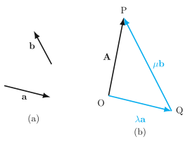
Figure 3.8 in the NCERT textbook is the visual foundation for the idea of resolving a vector into components along two given directions. It is not about the usual $x$ and $y$ axes; it is about breaking a vector into parts that lie along two non-collinear (non-parallel) vectors, $\mathbf{a}$ and $\mathbf{b}$ .

The figure has two parts. In part (a), you see two arrows, $\mathbf{a}$ and $\mathbf{b}$ , drawn from a common starting point. They are not parallel — they point in different directions. This is the "basis" you will use for the resolution. In part (b), the scene changes. A third vector, $\mathbf{A}$ , is introduced. Its tail is placed at the same starting point as $\mathbf{a}$ and $\mathbf{b}$ , and its head is at a point labelled $Q$ . The key geometric construction is a triangle: from the head of $\mathbf{A}$ (point $Q$ ), a line is drawn parallel to $\mathbf{b}$ until it meets the line along $\mathbf{a}$ at a point $O$ . Similarly, a line is drawn from $Q$ parallel to $\mathbf{a}$ until it meets the line along $\mathbf{b}$ at a point $P$ . The result is a parallelogram (or, equivalently, the triangle $OQP$ ) that shows $\mathbf{A}$ as the diagonal.

What this triangle teaches is that any vector $\mathbf{A}$ can be expressed as the sum of two scaled versions of $\mathbf{a}$ and $\mathbf{b}$ . The scaling factors are real numbers, $\lambda$ and $\mu$ . The vector from the origin to $O$ is $\lambda \mathbf{a}$ , and the vector from the origin to $P$ is $\mu \mathbf{b}$ . The vector $\mathbf{A}$ is then the diagonal of the parallelogram formed by these two scaled vectors, which is exactly their sum.

\mathbf{A} = \lambda \mathbf{a} + \mu \mathbf{b}

Here, $\lambda$ and $\mu$ are scalar components of $\mathbf{A}$ along the directions of $\mathbf{a}$ and $\mathbf{b}$ , respectively. The physical idea is that a single vector can be replaced by two perpendicular (or, in this general case, non-perpendicular) vectors that, when added head-to-tail, give the original vector. This is the core of resolution of vectors — the reverse operation of vector addition.

Watch out

The vectors $\mathbf{a}$ and $\mathbf{b}$ must be non-collinear (not parallel). If they were parallel, you could only ever produce vectors along that single line, and you could never reach a point $Q$ that lies off that line. The triangle construction would collapse. …

Figure 3.9(a) Unit vectors î, ĵ and k̂ lie along the x-, y-, and z-axes, each drawn as a short arrow near the origin overlapping the longer axis line. (b) Vector A resolved into components A1 (along the x-axis) and A2 (along the y-axis), shown with dashed construction lines from A's head to each axis. (c) The same vector A expressed as Axî + Ayĵ, with the angle θ it makes with the x-axis marked at O.

Drawn by us to help you understand the concept clearly, and verified to make sure it's accurate. For exams, practice from your NCERT textbook's own diagram.

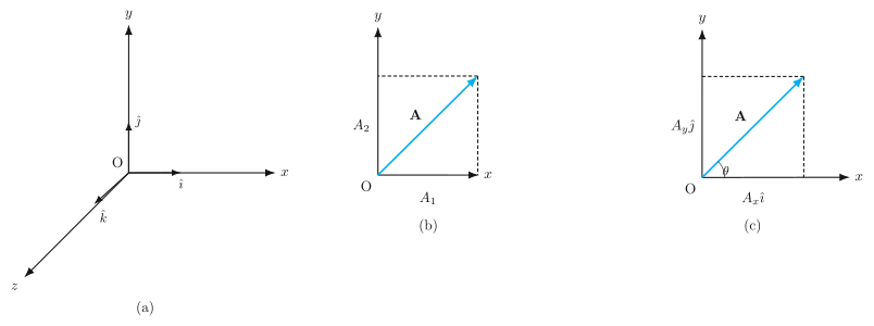
The figure has three panels, each building on the last. Panel (a) shows the standard right-handed coordinate system: three mutually perpendicular axes labelled $x$ , $y$ , and $z$ . Along each axis sits a unit vector — $\hat{i}$ along $x$ , $\hat{j}$ along $y$ , and $\hat{k}$ along $z$ . Each of these has length 1 and points in the positive direction of its axis. This is the stage on which all vector work in three dimensions happens.

Panel (b) zooms in to the $x$ – $y$ plane. A vector $\vec{A}$ is drawn as a diagonal arrow from the origin to some point. From the tip of $\vec{A}$ , dashed lines drop perpendicularly to the $x$ -axis and the $y$ -axis. The foot of the perpendicular on the $x$ -axis marks the scalar component $A_x$ ; the foot on the $y$ -axis marks $A_y$ . These are the rectangular components — the projections of $\vec{A}$ onto the two axes. The vector itself is the hypotenuse of the right triangle formed by $A_x$ and $A_y$ .

Panel (c) makes the connection explicit. The same vector $\vec{A}$ is now written as the sum of two perpendicular vectors: $A_x \hat{i}$ (the component along $x$ , scaled by the unit vector) and $A_y \hat{j}$ (the component along $y$ ). The angle $\theta$ that $\vec{A}$ makes with the positive $x$ -axis is marked. This panel shows the key idea: any vector in the plane can be built from two perpendicular building blocks.

Important

The central result the figure teaches is the resolution of a vector into rectangular components. For a vector $\vec{A}$ in the $x$ – $y$ plane making an angle $\theta$ with the $x$ -axis:

\vec{A} = A_x \hat{i} + A_y \hat{j}

where

$A_x = A \cos\theta$ is the scalar component along $x$ ,
$A_y = A \sin\theta$ is the scalar component along $y$ ,
$A = |\vec{A}| = \sqrt{A_x^2 + A_y^2}$ is the magnitude,
$\theta = \tan^{-1}(A_y / A_x)$ gives the direction. …

Figure 3.9.dA vector A resolved into three-dimensional components Ax, Ay, and Az along the x-, y-, and z-axes: A is drawn as the space diagonal of a dashed rectangular parallelepiped (box), with angles alpha, beta, and gamma marked at the origin between A and the x-, y-, and z-axes respectively, and the box's width, height, and depth also shown as separate labeled double-headed measurement brackets outside the box.

Fig. 3.9.d — A vector A resolved into three-dimensional components Ax, Ay, and Az along the x-, y-, and z-axes: A is drawn as the space diagonal of a dashed rectangular parallelepiped (box), with angles alpha, beta, and gamma marked at the origin between A and the x-, y-, and z-axes respectively, and the box's width, height, and depth also shown as separate labeled double-headed measurement brackets outside the box.

Drawn by us to help you understand the concept clearly, and verified to make sure it's accurate. For exams, practice from your NCERT textbook's own diagram.

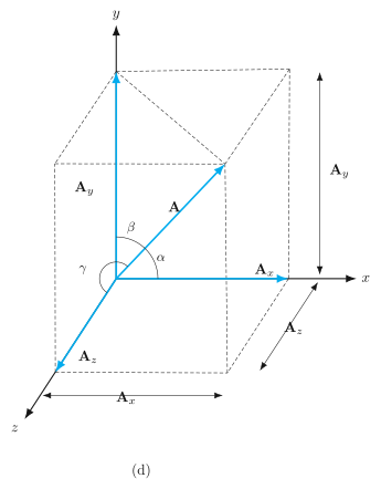
The figure shows a three-dimensional dashed box drawn on a set of $x$ , $y$ , $z$ axes. A single vector $\vec{A}$ runs from the origin along the diagonal of this box, ending at the opposite corner. From the tip of $\vec{A}$ , three dashed lines drop back to each axis, meeting the axes at the points $A_x$ , $A_y$ , and $A_z$ . At the origin, three angles are marked: $\alpha$ between $\vec{A}$ and the $x$ -axis, $\beta$ between $\vec{A}$ and the $y$ -axis, and $\gamma$ between $\vec{A}$ and the $z$ -axis.

The physical idea is straightforward: any vector in three-dimensional space can be broken into three mutually perpendicular pieces, one along each coordinate axis. The dashed box makes it clear that these three components are the sides of a rectangular parallelepiped whose diagonal is the original vector. The vector $\vec{A}$ is the sum of its three component vectors:

\vec{A} = A_x \hat{i} + A_y \hat{j} + A_z \hat{k}

where $\hat{i}$ , $\hat{j}$ , $\hat{k}$ are unit vectors along the $x$ , $y$ , and $z$ axes respectively. The magnitude of $\vec{A}$ is found from the three components by applying the Pythagorean theorem twice — once in the $xy$ -plane and then again with the $z$ -component:

|\vec{A}| = \sqrt{A_x^2 + A_y^2 + A_z^2}

The angles $\alpha$ , $\beta$ , $\gamma$ are called the direction angles of the vector. They relate the components to the magnitude through the direction cosines:

\cos\alpha = \frac{A_x}{|\vec{A}|}, \quad \cos\beta = \frac{A_y}{|\vec{A}|}, \quad \cos\gamma = \frac{A_z}{|\vec{A}|}

\cos^2\alpha + \cos^2\beta + \cos^2\gamma = 1

This last identity is a direct consequence of the magnitude formula: square each direction cosine and add them, and you get $\frac{A_x^2 + A_y^2 + A_z^2}{|\vec{A}|^2} = 1$ . It is a quick check that the three angles are consistent — if you know two of them, the third is determined up to sign. …

Start your 14-day free trial to unlock the full solution →

← Previous · 3.4Example 3.1 — Rain is falling vertically with a speed of 35m s⁻¹. Winds starts blowi…Next · 3.5 →Example 3.5 — A particle starts from origin at t = 0 with a velocity 5.0hatim/s and …