Physics · Ch 13 — Oscillations

Simple Harmonic Motion

13.3

Simple Harmonic Motion

The Meaning of Simple Harmonic Motion

Simple harmonic motion (SHM) is the most fundamental kind of oscillation. It occurs when the restoring force on a particle is directly proportional to its displacement from a fixed equilibrium position and always points towards that equilibrium. In other words, the force obeys Hooke's law: $F = -k x$ , where $k$ is a positive constant (the force constant) and $x$ is the displacement.

The negative sign is crucial — it tells you the force is a restoring force. If the particle is displaced to the right ( $x > 0$ ), the force pushes it left ( $F < 0$ ); if displaced left ( $x < 0$ ), the force pushes it right ( $F > 0$ ). The particle is always being pulled back toward $x = 0$ .

From Newton's second law, $F = m a$ , we get:

m a = -k x \quad \Rightarrow \quad a = -\frac{k}{m} x

Since $k$ and $m$ are constants for a given system, we can define a new constant $\omega^2 = k/m$ (where $\omega$ is the angular frequency). Then:

a = -\omega^2 x

This is the differential equation of SHM. It says that the acceleration is proportional to the negative of the displacement. The solution to this equation — the function $x(t)$ that describes the position at any time — is a sinusoidal function.

x(t) = A \cos(\omega t + \phi)

Here $A$ is the amplitude (maximum displacement from equilibrium), $\omega$ is the angular frequency (in rad/s), and $\phi$ is the initial phase (or phase constant), which determines where in the cycle the motion starts at $t = 0$ .

Properties of Simple Harmonic Motion

The textbook lists three key properties that follow directly from the sinusoidal solution. Each one is derived below.

›Proof

Property I: The acceleration is proportional to the negative of the displacement.

Start with $x(t) = A \cos(\omega t + \phi)$ . Differentiate once to get velocity:

$v(t) = \frac{dx}{dt} = -A\omega \sin(\omega t + \phi)$

Differentiate again to get acceleration:

$a(t) = \frac{dv}{dt} = -A\omega^2 \cos(\omega t + \phi)$

But $A \cos(\omega t + \phi) = x(t)$ , so:

$a(t) = -\omega^2 x(t)$

This is exactly the defining relation $a = -\omega^2 x$ . So the property is not an extra condition — it is built into the sinusoidal form.

›Proof

Property II: The velocity is zero at the extreme positions and maximum at the equilibrium position.

From $v(t) = -A\omega \sin(\omega t + \phi)$ , the magnitude of velocity is $|v| = A\omega |\sin(\omega t + \phi)|$ .

At the extremes: $x = \pm A$ means $\cos(\omega t + \phi) = \pm 1$ , so $\sin(\omega t + \phi) = 0$ . Hence $v = 0$ .
At equilibrium: $x = 0$ means $\cos(\omega t + \phi) = 0$ , so $\sin(\omega t + \phi) = \pm 1$ . Hence $|v| = A\omega$ , the maximum speed.

The maximum speed is therefore $v_{\text{max}} = A\omega$ .

›Proof

Property III: The acceleration is zero at equilibrium and maximum at the extremes.

From $a(t) = -\omega^2 x(t)$ :

At equilibrium ( $x = 0$ ): $a = 0$ .
At extremes ( $x = \pm A$ ): $|a| = \omega^2 A$ , the maximum acceleration.

The direction of acceleration is always toward equilibrium (opposite to $x$ ), so at the right extreme ( $x = +A$ ) the acceleration is $-\omega^2 A$ (leftward), and at the left extreme ( $x = -A$ ) it is $+\omega^2 A$ (rightward).

The Phase and Initial Conditions

The quantity $(\omega t + \phi)$ is called the phase of the motion. It tells you the current state of the oscillator — where it is and which way it is moving. The constant $\phi$ is the phase constant (or initial phase), which is determined by the initial conditions: the position $x_0$ and velocity $v_0$ at $t = 0$ .

At $t = 0$ :

x_0 = A \cos \phi

v_0 = -A\omega \sin \phi

From these two equations you can solve for $A$ and $\phi$ :

A = \sqrt{x_0^2 + \left(\frac{v_0}{\omega}\right)^2}

\tan \phi = -\frac{v_0}{\omega x_0}

Watch out

When using $\tan \phi = -v_0/(\omega x_0)$ , be careful with the quadrant. The signs of $x_0$ and $v_0$ together determine which quadrant $\phi$ lies in. For example, if $x_0 > 0$ and $v_0 > 0$ , then $\tan \phi$ is negative, so $\phi$ is in the fourth quadrant (between $-\pi/2$ and $0$ ). Always check both $x_0$ and $v_0$ to get the correct $\phi$ .

The Period and Frequency …

Figure 13.3A particle vibrating back and forth about the origin of x-axis, between the limits +A and –A.

Fig. 13.3 — A particle vibrating back and forth about the origin of x-axis, between the limits +A and –A.

Drawn by us to help you understand the concept clearly, and verified to make sure it's accurate. For exams, practice from your NCERT textbook's own diagram.

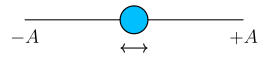
The figure shows a single horizontal line — the x-axis — with a small blue dot placed exactly at the origin. Two vertical tick marks are labelled: one at $x = -A$ on the left, one at $x = +A$ on the right. Beneath the axis, a double-headed arrow stretches from $-A$ to $+A$ , making it clear that the particle’s motion is confined to this interval. The particle itself is drawn at the centre, but the arrow tells you it does not stay there — it moves back and forth between the two extremes.

This is the simplest possible picture of simple harmonic motion (SHM). The blue dot represents a particle that oscillates symmetrically about the origin. The limits $\pm A$ are the amplitude of the motion: the maximum displacement from the equilibrium position (the origin). The double-headed arrow is a visual reminder that the motion is periodic and reversible — the particle goes from $+A$ to $-A$ and back again, over and over.

The physical idea is that the particle is under a restoring force that always points toward the origin and is proportional to the displacement. That force law is

F = -k x,

where $k$ is a positive constant (the force constant) and the minus sign means the force opposes the displacement. From Newton’s second law, $F = m a$ , this gives

m \frac{d^2 x}{d t^2} = -k x.

The solution to this differential equation is the displacement as a function of time:

x(t) = A \cos(\omega t + \phi),

where:

$A$ is the amplitude (the maximum displacement, shown in the figure as $\pm A$ ),
$\omega = \sqrt{k/m}$ is the angular frequency (radians per second),
$\phi$ is the initial phase (determines where in the cycle the particle starts).

The figure itself does not show the time axis — it is a snapshot of the spatial limits. But the formula above is the mathematical description of the motion that the figure introduces. The particle oscillates between $x = +A$ and $x = -A$ , and at any instant its position is given by the cosine function.

Important

The amplitude $A$ is the maximum displacement from equilibrium. It is not the total distance travelled in one cycle (which is $4A$ ). The particle moves from $+A$ to $-A$ (distance $2A$ ) and back to $+A$ (another $2A$ ), so one full oscillation covers $4A$ .

Watch out

Do not confuse the amplitude $A$ with the range of motion. The range is $2A$ (from $-A$ to $+A$ ). The amplitude is half that — the distance from equilibrium to either extreme. …

Figure 13.4The location of the particle in SHM at the discrete values t = 0, T/4, T/2, 3T/4, T, 5T/4.

Fig. 13.4 — The location of the particle in SHM at the discrete values t = 0, T/4, T/2, 3T/4, T, 5T/4.

Drawn by us to help you understand the concept clearly, and verified to make sure it's accurate. For exams, practice from your NCERT textbook's own diagram.

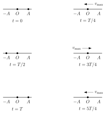
The figure is a sequence of six snapshots of a particle executing simple harmonic motion along a straight line. Each snapshot is a small number-line panel that runs from $-A$ (left) to $O$ (centre) to $A$ (right). The particle is shown as a dot at a specific position at a specific time. The times are chosen at quarter-period intervals: $t = 0$ , $T/4$ , $T/2$ , $3T/4$ , $T$ , and $5T/4$ .

At $t = 0$ , the particle sits at the extreme right position $x = +A$ . At $t = T/4$ , it has moved to the equilibrium point $x = 0$ , and the arrow on the dot indicates it is moving leftward with maximum speed $v_{\text{max}}$ . At $t = T/2$ , the particle is at the extreme left position $x = -A$ . At $t = 3T/4$ , it is back at $x = 0$ , now moving rightward with maximum speed $v_{\text{max}}$ . At $t = T$ , the particle has returned to $x = +A$ , completing one full cycle. The sixth panel, at $t = 5T/4$ , shows the particle again at $x = 0$ moving leftward with $v_{\text{max}}$ — the beginning of the next cycle.

The physical idea is that SHM is periodic motion about a central equilibrium point, with the speed greatest at the centre and zero at the extremes. The figure makes clear that the motion is symmetric: the particle takes the same time to go from $+A$ to $O$ as from $O$ to $-A$ , and the return journey is identical. The six panels are not a continuous curve; they are discrete instants that reveal the pattern of position and velocity over one full period.

The textbook uses this figure to introduce the displacement equation for SHM. If the particle starts at the extreme position $x = +A$ at $t = 0$ , the displacement as a function of time is given by a cosine function:

x(t) = A \cos(\omega t)

Here $A$ is the amplitude — the maximum displacement from equilibrium. $\omega$ is the angular frequency, related to the period $T$ by $\omega = 2\pi / T$ . At $t = 0$ , $\cos(0) = 1$ , so $x(0) = A$ , matching the first panel. At $t = T/4$ , $\omega t = \pi/2$ , $\cos(\pi/2) = 0$ , so $x = 0$ , matching the second panel. At $t = T/2$ , $\omega t = \pi$ , $\cos(\pi) = -1$ , so $x = -A$ , matching the third panel. The pattern continues, and the sixth panel at $t = 5T/4$ corresponds to $\omega t = 5\pi/2$ , $\cos(5\pi/2) = 0$ , again at $x = 0$ .

The velocity is obtained by differentiating $x(t)$ :

v(t) = \frac{dx}{dt} = -A\omega \sin(\omega t)

The magnitude of the maximum velocity is $v_{\text{max}} = A\omega$ . At $t = T/4$ , $\sin(\pi/2) = 1$ , so $v = -A\omega$ , which is $v_{\text{max}}$ directed leftward (negative sign). At $t = 3T/4$ , $\sin(3\pi/2) = -1$ , so $v = +A\omega$ , $v_{\text{max}}$ directed rightward. The figure's arrows on the panels at $t = T/4$ , $3T/4$ , and $5T/4$ directly illustrate these velocity directions. …

Figure 13.5Displacement as a continuous function of time for simple harmonic motion.

Fig. 13.5 — Displacement as a continuous function of time for simple harmonic motion.

Drawn by us to help you understand the concept clearly, and verified to make sure it's accurate. For exams, practice from your NCERT textbook's own diagram.

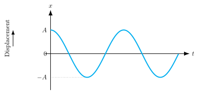
Fig. 13.5 is the first graph a student sees when learning simple harmonic motion (SHM), and it captures the entire essence of the motion in a single curve. The horizontal axis is time $t$ , the vertical axis is displacement $x$ from the equilibrium position. The curve is a smooth cosine wave that starts at the maximum positive displacement $x = +A$ at $t = 0$ , then falls, crosses zero, reaches the negative extreme $x = -A$ , turns around, and returns to $+A$ — repeating this cycle indefinitely.

Two dashed horizontal guide lines are drawn at $x = +A$ and $x = -A$ , marking the two extreme positions of the motion. These are the turning points where the particle momentarily stops before reversing direction. The curve itself is continuous and has no sharp corners — this tells you that the velocity changes smoothly, which is the hallmark of a restoring force that is proportional to displacement.

Note

The choice of a cosine function (rather than sine) is not accidental. Starting at $+A$ at $t=0$ is the natural description when the particle is released from rest at the extreme position. If the motion started from the equilibrium position moving upward, a sine function would be more natural.

The physical idea this figure teaches is that SHM is periodic and sinusoidal. The displacement does not just go back and forth — it does so in a way that can be described by a single trigonometric function. The smoothness of the curve reflects the fact that the acceleration is always directed toward the equilibrium point and is proportional to the displacement itself.

The key formula the textbook develops alongside this figure is the displacement equation for SHM:

x(t) = A \cos(\omega t + \phi)

For the specific case shown in Fig. 13.5, the initial phase $\phi = 0$ , so the equation simplifies to:

x(t) = A \cos(\omega t)

Here:

$x(t)$ is the displacement from equilibrium at time $t$ .
$A$ is the amplitude — the maximum displacement from equilibrium (the distance from $x=0$ to either dashed guide line).
$\omega$ is the angular frequency, measured in radians per second. It tells you how fast the oscillation occurs: one full cycle corresponds to $\omega t$ increasing by $2\pi$ radians.
$\omega t$ is the phase of the motion at time $t$ (with $\phi = 0$ ).

Watch out

Do not confuse angular frequency $\omega$ with ordinary frequency $f$ . They are related by $\omega = 2\pi f$ , but $\omega$ is measured in rad/s while $f$ is in Hz (cycles per second). The graph in Fig. 13.5 does not show $\omega$ directly — you infer it from the time period $T$ , which is the horizontal distance between two successive peaks (or troughs). The relation is $\omega = 2\pi / T$ . …

Figure 13.6The meaning of standard symbols in Eq. (13.4).

Fig. 13.6 — The meaning of standard symbols in Eq. (13.4).

Drawn by us to help you understand the concept clearly, and verified to make sure it's accurate. For exams, practice from your NCERT textbook's own diagram.

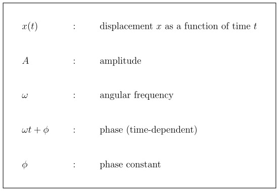
Fig. 13.6 is a visual key — a labelled legend — for the standard symbols that appear in the equation of simple harmonic motion. It does not show a graph or a moving object. Instead, it is a boxed reference that tells you, at a glance, what each symbol in the displacement equation physically means.

The figure lists five quantities, each with a short label:

$x(t)$ — displacement (the position of the oscillating particle measured from the equilibrium point, as a function of time)
$A$ — amplitude (the maximum displacement from equilibrium; the size of the oscillation)
$\omega$ — angular frequency (how fast the oscillation cycles, in radians per second)
$\omega t + \phi$ — phase (the argument of the sine or cosine function; it tells you where in the cycle the particle is at any time $t$ )
$\phi$ — phase constant (the initial phase at $t = 0$ ; it determines where in the cycle the motion starts)

The central formula that this figure supports is the displacement equation for simple harmonic motion:

x(t) = A \cos(\omega t + \phi)

Here, $x(t)$ is the displacement at time $t$ , $A$ is the amplitude, $\omega$ is the angular frequency, and $\phi$ is the phase constant. The quantity $\omega t + \phi$ is the phase. The figure exists to make sure you never confuse these symbols — each one has a distinct physical role.

Important

The phase $\omega t + \phi$ is not a separate symbol; it is the combination that appears inside the cosine. The phase constant $\phi$ is just the value of the phase when $t = 0$ .

The textbook uses this figure to anchor the meaning of every term before moving on to velocity, acceleration, and energy. Without this clear labelling, students often mix up amplitude and displacement, or think the phase constant is the same as the phase. The figure prevents that confusion by showing each symbol in isolation, with its definition right next to it. …

Figure 13.7.aA plot of displacement vs time with φ = 0. Curves 1 and 2 are for two different amplitudes A and B.

Fig. 13.7.a — A plot of displacement vs time with φ = 0. Curves 1 and 2 are for two different amplitudes A and B.

Drawn by us to help you understand the concept clearly, and verified to make sure it's accurate. For exams, practice from your NCERT textbook's own diagram.

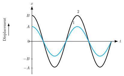
The figure is a displacement–time graph for two simple harmonic oscillators. The horizontal axis is time $t$ , and the vertical axis is displacement $x(t)$ . Both curves are cosine waves that start at $t = 0$ with their maximum positive displacement — that is, the phase constant $\phi$ is zero for both. Curve 1 (shown in blue, smaller amplitude) has amplitude $A$ , and curve 2 (shown in black, larger amplitude) has amplitude $B$ , with $B > A$ . The two curves are perfectly in phase: they reach their maxima, cross zero, and hit their minima at exactly the same instants. The only difference is the vertical stretch.

The physical idea is straightforward: for a given phase constant, the amplitude alone determines how far the oscillator swings from equilibrium. Both oscillators have the same angular frequency $\omega$ (the curves have the same period), so they move together in time — they are synchronous. The figure makes clear that amplitude is a scaling factor on the displacement, not something that changes the timing of the motion.

The textbook uses this figure to introduce the standard equation for simple harmonic motion:

x(t) = A \cos(\omega t + \phi)

Here $x(t)$ is the displacement at time $t$ , $A$ is the amplitude (maximum displacement from equilibrium), $\omega$ is the angular frequency (in rad/s), and $\phi$ is the phase constant (in radians). In the figure, $\phi = 0$ , so the equation reduces to $x(t) = A \cos(\omega t)$ for the smaller curve and $x(t) = B \cos(\omega t)$ for the larger one. The cosine function ensures that at $t = 0$ , $x(0) = A$ (or $B$ ) — the oscillator starts at its extreme positive position. …

Figure 13.7.bCurves 3 and 4 are for φ = 0 and -π/4 respectively; amplitude A same for both.

Fig. 13.7.b — Curves 3 and 4 are for φ = 0 and -π/4 respectively; amplitude A same for both.

Drawn by us to help you understand the concept clearly, and verified to make sure it's accurate. For exams, practice from your NCERT textbook's own diagram.

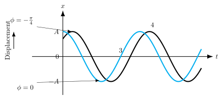
The figure is a displacement–time graph that shows two simple harmonic motions of the same amplitude $A$ but different phases. The horizontal axis is time $t$ , the vertical axis is displacement $x(t)$ . Both curves are cosine functions, so each starts at $t=0$ with a value determined by its phase.

Curve 3 (blue) has phase $\phi = 0$ . Its equation is $x(t) = A \cos(\omega t + 0) = A \cos(\omega t)$ . At $t=0$ , the displacement is $x(0) = A \cos 0 = A$ , the maximum positive value. The curve begins at the peak and then falls toward zero, crossing the time axis at $t = T/4$ (where $T$ is the period), reaching $-A$ at $t = T/2$ , and so on.

Curve 4 (black) has phase $\phi = -\pi/4$ . Its equation is $x(t) = A \cos(\omega t - \pi/4)$ . At $t=0$ , the displacement is $x(0) = A \cos(-\pi/4) = A/\sqrt{2}$ , about 0.707 times the amplitude. The curve starts at this positive value, not at the peak. It reaches its maximum $A$ later, at the time when $\omega t - \pi/4 = 0$ , i.e., $t = \pi/(4\omega) = T/8$ . So the black curve is shifted to the right relative to the blue curve — it lags behind by a time interval $\Delta t = \pi/(4\omega) = T/8$ .

Note

A negative phase $\phi$ means the motion starts later than the $\phi=0$ case. The shift in time is $\Delta t = -\phi/\omega$ . For $\phi = -\pi/4$ , the delay is $T/8$ .

The key formula the textbook develops with this figure is the general equation for simple harmonic motion:

x(t) = A \cos(\omega t + \phi)

Here $A$ is the amplitude (maximum displacement from equilibrium), $\omega$ is the angular frequency (in rad/s), $t$ is time, and $\phi$ is the initial phase (or phase constant) — the angle at $t=0$ . The period $T = 2\pi/\omega$ and frequency $f = 1/T = \omega/(2\pi)$ . …

Figure 13.8Plots for φ = 0 for two different periods.

Fig. 13.8 — Plots for φ = 0 for two different periods.

Drawn by us to help you understand the concept clearly, and verified to make sure it's accurate. For exams, practice from your NCERT textbook's own diagram.

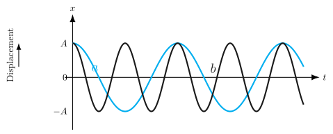
Figure 13.8 in the NCERT textbook is a simple but powerful visual: it places two cosine curves on the same set of axes, both starting from the same maximum displacement at $t = 0$ . The horizontal axis is time $t$ , and the vertical axis is displacement $x(t)$ . Both curves have the same amplitude $A$ — they reach the same peak height and the same trough depth. The difference is in how quickly they oscillate.

Curve a (shown in blue) has period $T$ . It completes one full to-and-fro motion — from $+A$ down to $-A$ and back to $+A$ — in time $T$ . Curve b (shown in black) has period $T/2$ . It goes through two complete cycles in the same time that curve a takes for one. The caption says "Plots for $\phi = 0$ for two different periods." The phase constant $\phi = 0$ means both curves start at $x = +A$ at $t = 0$ , so they are in step at the beginning. The only difference is the period, and the figure makes that difference immediately visible: curve b is twice as "squashed" horizontally.

Note

The phase constant $\phi$ is set to zero here so that the effect of changing the period is isolated. If $\phi$ were non-zero, the curves would also be shifted left or right, which would distract from the main point — that period alone controls how fast the oscillation repeats.

The physical idea is straightforward: the period $T$ is the time for one complete oscillation. A system with a smaller period oscillates faster. In the figure, curve b completes two oscillations in the time curve a completes one, so its period is half as large. This is not just a mathematical curiosity — it reflects real physics. A stiffer spring or a lighter mass gives a shorter period; a pendulum on a shorter string swings faster. The figure trains you to read that information directly from a graph.

The key formula that this figure illustrates is the displacement function for simple harmonic motion:

x(t) = A \cos(\omega t + \phi)

Here $A$ is the amplitude (the maximum displacement from equilibrium), $\omega$ is the angular frequency, $t$ is time, and $\phi$ is the phase constant (initial phase). For the two curves in Fig. 13.8, $\phi = 0$ , so the equation simplifies to $x(t) = A \cos(\omega t)$ .

The angular frequency $\omega$ is related to the period $T$ by $\omega = 2\pi / T$ . For curve a, $\omega_a = 2\pi / T$ . For curve b, $T_b = T/2$ , so $\omega_b = 2\pi / (T/2) = 4\pi / T = 2\omega_a$ . The angular frequency of curve b is twice that of curve a. This is why curve b oscillates twice as fast — its cosine argument $\omega t$ changes twice as quickly.

Watch out

A common mistake is to confuse angular frequency $\omega$ (radians per second) with ordinary frequency $f$ (cycles per second). They are related by $\omega = 2\pi f$ , and $f = 1/T$ . In the figure, curve b has $f_b = 2/T$ and $\omega_b = 4\pi/T$ , while curve a has $f_a = 1/T$ and $\omega_a = 2\pi/T$ . The factor of $2\pi$ is crucial.

The figure also reinforces the meaning of the cosine function itself. At $t = 0$ , $\cos(0) = 1$ , so $x(0) = A$ . At $t = T/4$ , $\cos(\pi/2) = 0$ , so $x = 0$ (the equilibrium crossing). At $t = T/2$ , $\cos(\pi) = -1$ , so $x = -A$ (the opposite extreme). These key points — maximum, zero, minimum — are the same for both curves, but they occur at different times because the periods differ. For curve b, the first zero crossing happens at $t = T/8$ , not $T/4$ , and the first negative peak at $t = T/4$ , not $T/2$ . …

Start your 14-day free trial to unlock the full solution →

← Previous · 13.2.2Example 13.2 — Which of the following functions of time represent (a) periodic and (b…Next · 13.3 →Example 13.3 — Which of the following functions of time represent (a) simple harmonic…