Economics · Ch 10 — The Theory of the Firm under Perfect Competition

Input Prices

10.5.2

Input Prices

Input Prices and the Supply Curve

A change in the price of an input — say, a rise in the wage rate of labour — directly raises the firm’s cost of production. When an input becomes more expensive, the firm’s average cost at every output level increases. More importantly, the marginal cost also rises at every output level. This means the entire MC curve shifts upward (or, equivalently, to the left).

Why does a higher MC shift the supply curve? Recall that a perfectly competitive firm’s short-run supply curve is exactly the rising portion of its MC curve above the minimum AVC. If the MC curve moves upward, then at any given market price the firm will now produce fewer units than before. Graphically, the supply curve shifts to the left.

Watch out

Do not confuse a movement along the supply curve (caused by a change in the good’s own price) with a shift of the supply curve (caused by a change in input prices, technology, or other non-price factors). A rise in input prices shifts the entire supply curve leftward.

Note

Impact of a unit tax on supply

A unit tax is a tax the government imposes on each unit of output that a firm sells. For example, if the unit tax is Rs 2 and the firm produces and sells 10 units, the total tax it must pay is $10 \times \text{Rs }2 = \text{Rs }20$ .

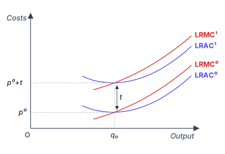
How does the firm's long-run supply curve change when such a tax is imposed? Before the tax, let the firm's long-run marginal and average cost curves be $LRMC_0$ and $LRAC_0$ . Once a unit tax of Rs $t$ is levied, the firm pays an extra Rs $t$ on every unit it produces, so both its long-run average cost and its long-run marginal cost rise by exactly Rs $t$ at every level of output. This gives the new curves $LRMC_1$ and $LRAC_1$ , each lying Rs $t$ above the original curve.

Since the firm's long-run supply curve is the part of the $LRMC$ curve lying above $LRAC$ , this upward shift moves the long-run supply curve upward, or equivalently to the left. At any given market price, the firm now supplies fewer units than it did before the tax.

Figure 4.11Cost Curves and the Unit Tax. LRAC⁰ and LRMC⁰ are, respectively, the long run average cost curve and the long run marginal cost curve of a firm before a unit tax is imposed. LRAC¹ and LRMC¹ are, respectively, the long run average cost curve and the long run marginal cost curve of a firm after a unit tax of Rs t is imposed.

Fig. 4.11 — Cost Curves and the Unit Tax. LRAC⁰ and LRMC⁰ are, respectively, the long run average cost curve and the long run marginal cost curve of a firm before a unit tax is imposed. LRAC¹ and LRMC¹ are, respectively, the long run average cost curve and the long run marginal cost curve of a firm after a unit tax of Rs t is imposed.

Drawn by us to help you understand the concept clearly, and verified to make sure it's accurate. For exams, practice from your NCERT textbook's own diagram.

The figure plots two sets of long-run cost curves for a single firm, before and after a unit tax. The horizontal axis measures output $q$ , and the vertical axis measures cost in rupees. Before the tax, the firm faces the long-run average cost curve $LRAC^0$ and the long-run marginal cost curve $LRMC^0$ . After a unit tax of Rs $t$ is imposed, these curves shift upward to $LRAC^1$ and $LRMC^1$ .

The core idea is that a unit tax — a fixed amount per unit of output — acts exactly like an increase in the firm's variable cost. Because the tax is levied on each unit produced, it raises both average cost and marginal cost by the same constant amount $t$ at every output level. This means the vertical distance between $LRAC^1$ and $LRAC^0$ is exactly Rs $t$ , and the same holds for the marginal cost curves: $LRMC^1$ lies Rs $t$ above $LRMC^0$ at every quantity.

Why does the tax shift both curves by the same amount? Average cost includes total variable cost plus total fixed cost, divided by output. A unit tax adds $t$ to the cost of each unit, so average cost rises by $t$ . Marginal cost is the cost of producing one more unit; since each extra unit now costs an additional Rs $t$ in tax, marginal cost also rises by $t$ . The shapes of the curves do not change — they are simply translated upward.

Important

A unit tax shifts both the long-run average cost curve and the long-run marginal cost curve vertically upward by exactly the amount of the tax $t$ at every output level. The curves retain their original shapes.

The textbook uses this figure to derive the key formula for the firm's long-run supply curve under a unit tax. In long-run equilibrium under perfect competition, a firm produces where price equals long-run marginal cost, and price also equals the minimum of long-run average cost. Before the tax, the equilibrium price $p^0$ equals the minimum of $LRAC^0$ , and the firm produces at the output where $LRMC^0$ equals that price. After the tax, the new long-run equilibrium price $p^1$ must equal the minimum of $LRAC^1$ , which is $t$ rupees higher than the old minimum. The firm's new output is where $LRMC^1$ equals $p^1$ .

p^1 = p^0 + t

…

Figure 4.12Supply Curves and Unit Tax. S⁰ is the supply curve of a firm before a unit tax is imposed. After a unit tax of Rs t is imposed, S¹ represents the supply curve of the firm.

Fig. 4.12 — Supply Curves and Unit Tax. S⁰ is the supply curve of a firm before a unit tax is imposed. After a unit tax of Rs t is imposed, S¹ represents the supply curve of the firm.

Drawn by us to help you understand the concept clearly, and verified to make sure it's accurate. For exams, practice from your NCERT textbook's own diagram.

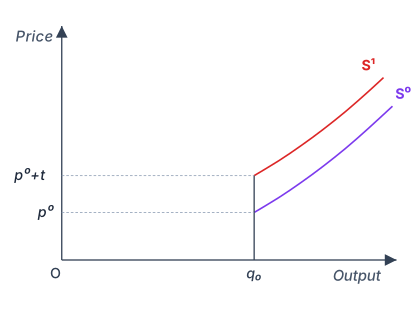
The figure plots the supply curve of a perfectly competitive firm on a graph with quantity ( $q$ ) on the horizontal axis and price/cost ( $P$ ) on the vertical axis. Two upward-sloping supply curves are drawn: the original supply curve labelled $S^0$ and a new supply curve labelled $S^1$ that lies vertically above $S^0$ by a constant distance.

The key idea is simple: a unit tax (also called a per-unit tax or specific tax) of Rs $t$ is imposed on the firm. This tax is a fixed amount the firm must pay to the government for every unit it produces and sells. Because the firm now has to cover this extra cost per unit, its supply behaviour changes.

Before the tax, the firm’s supply curve $S^0$ is its long run marginal cost (LRMC) curve above the minimum of its long run average cost (LRAC). After the tax, the firm’s effective marginal cost at every output level rises by exactly Rs $t$ . The new supply curve $S^1$ is therefore the original MC curve shifted upward by $t$ — at each quantity, the price the firm now requires to supply that quantity is higher by the amount of the tax.

Watch out

A common mistake is to think the supply curve shifts leftward (a horizontal shift). It does not. The shift is vertical — the same quantity is supplied only at a higher price. The curve moves up, not left.

The textbook uses this figure to derive the central formula for the effect of a unit tax on the firm’s supply. If the original supply function is $q = S(P)$ , then after a tax of Rs $t$ per unit, the new supply function becomes:

q = S(P - t)

Here, $P$ is the market price the firm receives from selling its output. But the firm must pay Rs $t$ to the government for each unit sold, so the net price the firm actually keeps is $P - t$ . The firm decides how much to supply based on this net price, not the gross market price. So to find the quantity supplied at a given market price $P$ , you plug the net price $P - t$ into the original supply function.

Equivalently, you can think of the inverse supply curve. If the original inverse supply is $P = MC(q)$ , then after the tax the firm’s supply condition becomes $P = MC(q) + t$ . The market price must now cover both the marginal cost of production and the tax. This is exactly the vertical shift shown in the figure: at each quantity $q$ , the new supply price is the old supply price plus $t$ . …

Start your 14-day free trial to unlock the full solution →

← Previous · 10.5.1Technological Progress Next · 10.6 →Market Supply Curve