Mathematics · Ch 13 — Statistics

Mean Deviation for Grouped Data

13.4.2

Mean Deviation for Grouped Data

Data can be grouped in two ways: as a discrete frequency distribution (where each observation is a distinct value with its own frequency) or as a continuous frequency distribution (where data is divided into class intervals). The method for finding mean deviation differs slightly between the two, but the core idea remains the same — we measure the average absolute distance of the data from a central value.

(a) Discrete Frequency Distribution

Suppose we have $n$ distinct values $x_1, x_2, \dots, x_n$ occurring with frequencies $f_1, f_2, \dots, f_n$ respectively. The data is arranged as:

$x$	$x_1$	$x_2$	$x_3$	$\dots$	$x_n$
$f$	$f_1$	$f_2$	$f_3$	$\dots$	$f_n$

Here $N = \sum_{i=1}^{n} f_i$ is the total number of observations.

(i) Mean Deviation About the Mean

Step 1 — Find the mean.

The mean $\bar{x}$ of the grouped data is:

\bar{x} = \frac{\sum_{i=1}^{n} f_i x_i}{\sum_{i=1}^{n} f_i} = \frac{1}{N} \sum_{i=1}^{n} f_i x_i

Step 2 — Find absolute deviations from the mean.

For each observation $x_i$ , compute $|x_i - \bar{x}|$ .

Step 3 — Find the weighted mean of these absolute deviations.

Multiply each absolute deviation by its frequency, sum them up, and divide by $N$ :

\text{M.D.}(\bar{x}) = \frac{\sum_{i=1}^{n} f_i |x_i - \bar{x}|}{\sum_{i=1}^{n} f_i} = \frac{1}{N} \sum_{i=1}^{n} f_i |x_i - \bar{x}|

Watch out

The deviations are taken in absolute value — signs are ignored. If you sum the signed deviations $f_i(x_i - \bar{x})$ , you will always get zero. That is why we use absolute values.

Example 4 — Find the mean deviation about the mean for:

$x_i$	2	5	6	8	10	12
$f_i$	2	8	10	7	8	5

Solution. First compute the mean:

\bar{x} = \frac{\sum f_i x_i}{N} = \frac{2(2) + 5(8) + 6(10) + 8(7) + 10(8) + 12(5)}{2+8+10+7+8+5} = \frac{4+40+60+56+80+60}{40} = \frac{300}{40} = 7.5

Now compute $|x_i - \bar{x}|$ and $f_i|x_i - \bar{x}|$ :

$x_i$	$f_i$	$f_i x_i$	$\lvert x_i - 7.5 \rvert$	$f_i\lvert x_i - 7.5 \rvert$
2	2	4	5.5	11
5	8	40	2.5	20
6	10	60	1.5	15
8	7	56	0.5	3.5
10	8	80	2.5	20
12	5	60	4.5	22.5
Total	40	300		92

\text{M.D.}(\bar{x}) = \frac{1}{N} \sum f_i |x_i - \bar{x}| = \frac{1}{40} \times 92 = 2.3

(ii) Mean Deviation About the Median

Step 1 — Find the median.

Arrange the observations in ascending order. Compute cumulative frequencies. The median is the value of the observation whose cumulative frequency is equal to or just greater than $N/2$ .

Note

If $N$ is even, the median is the average of the $\frac{N}{2}$ -th and $\left(\frac{N}{2}+1\right)$ -th observations. Both lie in the same class when the cumulative frequency first reaches or exceeds $N/2$ .

Step 2 — Find absolute deviations from the median.

For each $x_i$ , compute $|x_i - M|$ , where $M$ is the median.

Step 3 — Find the weighted mean of these absolute deviations.

\text{M.D.}(M) = \frac{\sum_{i=1}^{n} f_i |x_i - M|}{\sum_{i=1}^{n} f_i} = \frac{1}{N} \sum_{i=1}^{n} f_i |x_i - M|

Example 5 — Find the mean deviation about the median for:

$x_i$	3	6	9	12	13	15	21	22
$f_i$	3	4	5	2	4	5	4	3

Solution. The data is already in ascending order. Compute cumulative frequencies:

$x_i$	3	6	9	12	13	15	21	22
$f_i$	3	4	5	2	4	5	4	3
c.f.	3	7	12	14	18	23	27	30

$N = 30$ , so $N/2 = 15$ . The 15th and 16th observations both lie in the cumulative frequency 18, which corresponds to $x_i = 13$ . Therefore:

M = \frac{13 + 13}{2} = 13

Now compute $|x_i - M|$ and $f_i|x_i - M|$ :

$x_i$	$\lvert x_i - 13 \rvert$	$f_i$	$f_i\lvert x_i - 13 \rvert$
3	10	3	30
6	7	4	28
9	4	5	20
12	1	2	2
13	0	4	0
15	2	5	10
21	8	4	32
22	9	3	27
Total		30	149

\text{M.D.}(M) = \frac{1}{30} \times 149 = 4.97

(b) Continuous Frequency Distribution

In a continuous frequency distribution, data is grouped into class intervals without gaps. For example:

Marks	0-10	10-20	20-30	30-40	40-50	50-60
Students	12	18	27	20	17	6

The key assumption: the frequency in each class is centred at its mid-point. So we first find the mid-point $x_i$ of each class, then proceed exactly as for a discrete frequency distribution.

(i) Mean Deviation About the Mean

Step 1 — Find the mid-point $x_i$ of each class.

For a class $a-b$ , the mid-point is $\frac{a+b}{2}$ .

Step 2 — Compute the mean $\bar{x}$ .

Use the same formula as for discrete data:

\bar{x} = \frac{\sum f_i x_i}{\sum f_i} = \frac{1}{N} \sum f_i x_i

Step 3 — Compute absolute deviations $|x_i - \bar{x}|$ and their weighted sum.

Then:

\text{M.D.}(\bar{x}) = \frac{1}{N} \sum f_i |x_i - \bar{x}|

Example 6 — Find the mean deviation about the mean for:

Marks	10-20	20-30	30-40	40-50	50-60	60-70	70-80
Students	2	3	8	14	8	3	2

Solution. Compute mid-points and the required columns:

Class	$f_i$	$x_i$	$f_i x_i$	$\lvert x_i - 45 \rvert$	$f_i\lvert x_i - 45 \rvert$
10-20	2	15	30	30	60
20-30	3	25	75	20	60
30-40	8	35	280	10	80
40-50	14	45	630	0	0
50-60	8	55	440	10	80
60-70	3	65	195	20	60
70-80	2	75	150	30	60
Total	40		1800		400

\bar{x} = \frac{1800}{40} = 45

\text{M.D.}(\bar{x}) = \frac{1}{40} \times 400 = 10

Shortcut Method (Step-Deviation Method) for Mean Deviation About the Mean

When the mid-points are large, we can simplify the calculation of $\bar{x}$ using step deviations. This involves shifting the origin (choosing an assumed mean $a$ ) and changing the scale (dividing by a common factor $h$ ).

Define a new variable:

d_i = \frac{x_i - a}{h}

where $a$ is the assumed mean (usually a mid-point near the centre of the data) and $h$ is the common factor (the class width, if all classes have equal width).

Then the mean is:

\bar{x} = a + h \cdot \frac{\sum f_i d_i}{N}

Tip

The step-deviation method only simplifies the calculation of $\bar{x}$ . The rest of the procedure — finding $|x_i - \bar{x}|$ and then $\text{M.D.}(\bar{x})$ — remains exactly the same. You still need to compute the actual absolute deviations from the actual mean.

Example 6 using step-deviation method.

Take $a = 45$ (the mid-point of the 40-50 class) and $h = 10$ (the class width).

Class	$f_i$	$x_i$	$d_i = \frac{x_i - 45}{10}$	$f_i d_i$	$\lvert x_i - 45 \rvert$	$f_i\lvert x_i - 45 \rvert$
10-20	2	15	-3	-6	30	60
20-30	3	25	-2	-6	20	60
30-40	8	35	-1	-8	10	80
40-50	14	45	0	0	0	0
50-60	8	55	1	8	10	80
60-70	3	65	2	6	20	60
70-80	2	75	3	6	30	60
Total	40			0		400

\bar{x} = 45 + 10 \times \frac{0}{40} = 45

\text{M.D.}(\bar{x}) = \frac{400}{40} = 10

The result is identical, as expected.

(ii) Mean Deviation About the Median

The process is similar to the discrete case, but we must first find the median using the formula for continuous data.

Step 1 — Find the median class.

Arrange the data in ascending order (the classes are already in order). Compute cumulative frequencies. The median class is the class interval whose cumulative frequency is just greater than or equal to $N/2$ .

Step 2 — Apply the median formula.

\text{Median} = l + \frac{\frac{N}{2} - C}{f} \times h

where:

$l$ = lower limit of the median class
$f$ = frequency of the median class
$h$ = width of the median class
$C$ = cumulative frequency of the class just preceding the median class
$N$ = total frequency …

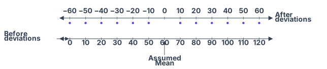
Figure 13.3Shifting the origin to the assumed mean (step-deviation method)

Fig. 13.3 — Shifting the origin to the assumed mean (step-deviation method)

Drawn by us to help you understand the concept clearly, and verified to make sure it's accurate. For exams, practice from your textbook's own diagram.

Fig. 13.3 is a visual of the core idea behind the step-deviation method: you can shift the origin of your number line to a convenient assumed mean, work with smaller numbers, and then shift back at the end.

The figure shows two aligned number lines, one above the other. The bottom line is the original data scale, running from 0 to 120. The top line is the deviation scale, running from −60 to 60. Each tick mark on the bottom line has a corresponding tick directly above it on the top line. The key alignment is at the value 60 on the bottom line: directly above it, on the top line, sits the deviation 0. An upward arrow labelled "Assumed Mean" points to 60 on the bottom line.

What this teaches is that subtracting the assumed mean $a$ from every observation $x_i$ is equivalent to sliding the entire number line leftwards so that the origin (0 on the deviation line) now sits at the assumed mean. The deviations $x_i - a$ are the new coordinates on the shifted line. If all these deviations also share a common factor $h$ (like all being multiples of 10), you can further scale them down by dividing by $h$ , giving the step-deviations $d_i = \frac{x_i - a}{h}$ . This is a change of scale on the number line, shown separately in Fig. 13.4.

The textbook uses this figure to introduce the step-deviation formula for the mean:

\bar{x} = a + h \cdot \frac{1}{N} \sum_{i=1}^{n} f_i d_i

Here, $a$ is the assumed mean (the point to which you shift the origin), $h$ is the common factor (the scale divisor), $d_i = \frac{x_i - a}{h}$ are the step-deviations, $f_i$ are the frequencies, and $N = \sum f_i$ is the total frequency. The formula says: compute the mean of the step-deviations, multiply by $h$ to undo the scaling, then add $a$ to undo the shift. The figure makes it clear that this is just a two-step translation of the number line — first a shift, then a rescaling — and that the mean follows the same transformation. …

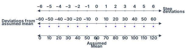
Figure 13.4Change of scale to step-deviations

Fig. 13.4 — Change of scale to step-deviations

Drawn by us to help you understand the concept clearly, and verified to make sure it's accurate. For exams, practice from your textbook's own diagram.

Fig. 13.4 is a visual explanation of the step-deviation method — a shortcut for calculating the mean of grouped data when the class intervals are equal. The figure shows three horizontal number lines, one above the other, all aligned vertically so that the same tick marks line up.

The bottom number line is the original raw scale, running from 0 to 120. This is the scale on which the actual data (mid-points of classes) live. The middle number line shows "deviations from assumed mean" — it runs from −60 to +60. Each tick on this line corresponds to the difference between a raw value and the assumed mean, which is chosen as 60. The indigo dots on each tick mark the actual deviation values. An upward arrow labelled "Assumed Mean" points to the 60 mark on the bottom scale, making it clear that the origin of the middle line has been shifted to that point.

The top number line shows "step deviations" — it runs from −6 to +6. This is the result of dividing every deviation from the middle line by a common factor (here, 10). So the step deviation is simply the deviation divided by the class width.

The key idea the figure teaches is that you can simplify calculations by first shifting the origin (subtracting an assumed mean) and then changing the scale (dividing by the common factor). This transforms the original mid-points $x_i$ into step deviations $d_i$ using:

d_i = \frac{x_i - a}{h}

where $a$ is the assumed mean (60 in the figure) and $h$ is the common factor (10 in the figure). The mean of the original data can then be recovered by reversing both transformations:

\bar{x} = a + h \cdot \frac{\sum f_i d_i}{N}

Here, $N = \sum f_i$ is the total frequency. The textbook uses this method to compute the mean for the data in Example 6 (marks of students), where $a = 45$ and $h = 10$ , and then finds the mean deviation about the mean using the usual formula:

\text{M.D.}(\bar{x}) = \frac{1}{N} \sum f_i |x_i - \bar{x}|

Note

The step-deviation method does not change the value of the mean deviation itself — it only simplifies the calculation of $\bar{x}$ . Once $\bar{x}$ is found, the deviations $|x_i - \bar{x}|$ are computed directly from the original mid-points, not from the step deviations.

Watch out

A common mistake is to think that the step deviations $d_i$ can be used directly in the mean deviation formula. They cannot — the mean deviation requires absolute differences from the actual mean $\bar{x}$ , not from the assumed mean. The step-deviation trick works only for computing $\bar{x}$ itself. …

Table 13.1Mean deviation about the mean (discrete distribution: x=2..12)

$x_i$	$f_i$	$f_ix_i$	$\lvert x_i-\bar{x} \rvert$	$f_i\lvert x_i-\bar{x} \rvert$
2	2	4	5.5	11
5	8	40	2.5	20
6	10	60	1.5	15
8	7	56	0.5	3.5
10	8	80	2.5	20

Table 13.2Discrete data with cumulative frequency row

$x_i$	3	6	9	12	13	15	21	22
$f_i$	3	4	5	2	4	5	4	3

Table 13.3Absolute deviations from the median

$\lvert x_i-M \rvert$	10	7	4	1	0	2	8	9
$f_i$	3	4	5	2	4	5	4	3

Table 13.4Mean deviation about the mean for grouped (continuous) data

Marks obtained	Number of students $f_i$	Mid-points $x_i$	$f_ix_i$	$\lvert x_i-\bar{x} \rvert$	$f_i\lvert x_i-\bar{x} \rvert$
10-20	2	15	30	30	60
20-30	3	25	75	20	60
30-40	8	35	280	10	80
40-50	14	45	630	0	0
50-60	8	55	440	10	80

Table 13.5Mean deviation by the step-deviation (shortcut) method

Marks obtained	Number of students $f_i$	Mid-points $x_i$	$d_i=\dfrac{x_i-45}{10}$	$f_id_i$	$\lvert x_i-\bar{x} \rvert$	$f_i\lvert x_i-\bar{x} \rvert$
10-20	2	15	$-3$	$-6$	30	60
20-30	3	25	$-2$	$-6$	20	60
30-40	8	35	$-1$	$-8$	10	80
40-50	14	45	0	0	0	0
50-60	8	55	1	8	10	80

Table 13.6Mean deviation about the median for grouped (continuous) data

Class	Frequency $f_i$	Cumulative frequency $c.f.$	Mid-points $x_i$	$\lvert x_i-\text{Med.} \rvert$	$f_i\lvert x_i-\text{Med.} \rvert$
0-10	6	6	5	23	138
10-20	7	13	15	13	91
20-30	15	28	25	3	45
30-40	16	44	35	7	112

Start your 14-day free trial to unlock the full solution →

← Previous · 13.4.1Example 3 — Find the mean deviation about the median for the following data: 3, 9,…Next · 13.4.2 →Example 4 — Find the mean deviation about the mean for the following data: | xᵢ | …