Physics · Ch 8 — Mechanical Properties of Solids

Applications of Elastic Behaviour of Materials

8.6

Applications of Elastic Behaviour of Materials

The Practical Power of Elastic Behaviour

The theory of elasticity is not just an abstract set of formulas — it is the engineering backbone of every structure you see around you. When a civil engineer designs a bridge, a skyscraper, or even a simple steel beam in a ceiling, they must ensure that the deformation under load stays within safe limits. The material must not only avoid permanent damage (plastic deformation) but also not deflect so much that the structure becomes unusable or unsafe.

The key insight is this: the elastic behaviour of a material — how it stretches, compresses, or bends under a force and then returns to its original shape — is what allows engineers to predict and control these deformations. By using the relations between stress and strain (Hooke's law, Young's modulus, shear modulus, bulk modulus), they can calculate exactly how much a given load will change the dimensions of a structural member.

Designing a Steel Rod: The Core Calculation

Consider the most straightforward application: a cylindrical rod of length $L$ and cross-sectional area $A$ , subjected to a tensile force $F$ along its axis. The rod will elongate by an amount $\Delta L$ . From the definition of Young's modulus $Y$ :

Y = \frac{\text{Tensile stress}}{\text{Tensile strain}} = \frac{F/A}{\Delta L / L}

Rearranging this gives the fundamental design equation:

\Delta L = \frac{F L}{A Y}

This single formula is the starting point for thousands of engineering decisions. It tells you that the elongation is directly proportional to the load $F$ and the original length $L$ , and inversely proportional to the area $A$ and the material's stiffness $Y$ .

Important

The elongation $\Delta L = \frac{F L}{A Y}$ is the master equation for axial deformation. Every structural design that involves tension or compression begins here.

The Three Design Constraints

When an engineer uses this equation, they are typically checking three things simultaneously:

Strength: The stress $\sigma = F/A$ must be well below the material's elastic limit (or yield strength). If the stress exceeds this limit, the material will undergo permanent plastic deformation and the structure will fail. A factor of safety (typically 2 to 5) is always applied.
Stiffness: The elongation $\Delta L$ must be small enough that the structure functions properly. A bridge that sags too much is unusable, even if it doesn't break. The equation $\Delta L = FL/AY$ directly gives this deflection.
Stability: For slender columns (compression members), there is a risk of buckling — a sudden sideways collapse that occurs at a stress far below the material's compressive strength. This is governed by Euler's formula (studied in higher mechanics), not by simple stress-strain relations.

Watch out

Do not confuse strength (the stress at which a material fails) with stiffness (Young's modulus $Y$ ). A material can be very strong (high breaking stress) but not very stiff (low $Y$ ), like many polymers. Conversely, a material can be very stiff (high $Y$ ) but brittle (low breaking strain), like glass.

The Steel Wire Example: A Step-by-Step Derivation

The textbook works through a classic problem to show how these ideas come together. Let us follow it carefully.

Problem: A steel wire of length $4.7\ \text{m}$ and cross-sectional area $3.0 \times 10^{-5}\ \text{m}^2$ stretches by the same amount as a copper wire of length $3.5\ \text{m}$ and cross-sectional area $4.0 \times 10^{-5}\ \text{m}^2$ under a given load. What is the ratio of Young's modulus of steel to that of copper?

Solution:

Let the common load be $F$ . For the steel wire:

\Delta L_{\text{steel}} = \frac{F L_s}{A_s Y_s}

For the copper wire:

\Delta L_{\text{copper}} = \frac{F L_c}{A_c Y_c}

The problem states that the elongations are equal: $\Delta L_{\text{steel}} = \Delta L_{\text{copper}}$ . Therefore:

\frac{F L_s}{A_s Y_s} = \frac{F L_c}{A_c Y_c}

The load $F$ cancels out. Rearranging to find the ratio $Y_s / Y_c$ :

\frac{Y_s}{Y_c} = \frac{L_s}{A_s} \times \frac{A_c}{L_c}

Substitute the given values:

\frac{Y_s}{Y_c} = \frac{4.7}{3.0 \times 10^{-5}} \times \frac{4.0 \times 10^{-5}}{3.5}

Simplify:

\frac{Y_s}{Y_c} = \frac{4.7 \times 4.0}{3.0 \times 3.5} = \frac{18.8}{10.5} \approx 1.79

Note

The units of area ( $\text{m}^2$ ) cancel out, as do the units of length ( $\text{m}$ ). The ratio is a pure number. This is always the case when comparing material properties — the geometry factors cancel, leaving only the intrinsic material stiffness ratio.

Answer: The ratio $Y_{\text{steel}} / Y_{\text{copper}} \approx 1.79$ . Steel is about 1.8 times stiffer than copper.

The Steel Rope Problem: A Second Worked Example

Problem: Two wires of diameter $d$ and $2d$ are made of the same material. They are loaded with the same force $F$ . What is the ratio of their elongations?

Solution:

Since the material is the same, $Y$ is identical for both wires. The cross-sectional area is proportional to the square of the diameter:

A_1 = \pi \left(\frac{d}{2}\right)^2 = \frac{\pi d^2}{4}, \quad A_2 = \pi \left(\frac{2d}{2}\right)^2 = \pi d^2

So $A_2 = 4 A_1$ .

Using $\Delta L = FL/AY$ , and assuming the lengths $L$ are the same:

\frac{\Delta L_1}{\Delta L_2} = \frac{F L / (A_1 Y)}{F L / (A_2 Y)} = \frac{A_2}{A_1} = \frac{4 A_1}{A_1} = 4

Answer: The thinner wire (diameter $d$ ) elongates four times as much as the thicker wire (diameter $2d$ ). This dramatically illustrates why structural members are made thick — doubling the diameter reduces the elongation by a factor of four.

Beyond Simple Tension: Bending of Beams

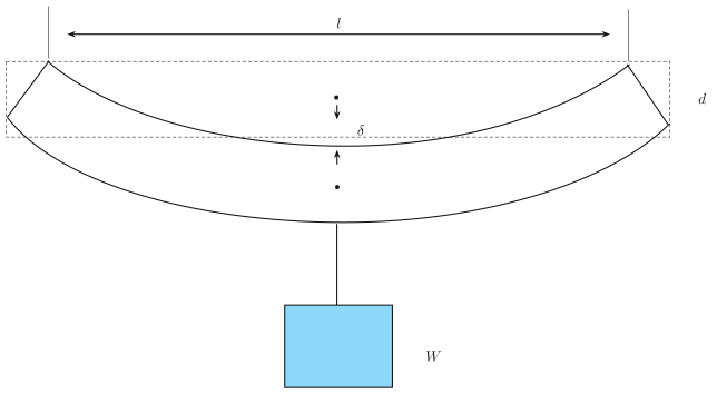
The same principles extend to more complex loading situations. Consider a beam supported at both ends with a load applied at the centre. The beam bends. The top surface compresses (shortens), the bottom surface stretches (elongates), and there is a neutral plane in the middle that experiences no change in length. …

Figure 8.6A beam supported at the ends and loaded at the centre.

Fig. 8.6 — A beam supported at the ends and loaded at the centre.

Drawn by us to help you understand the concept clearly, and verified to make sure it's accurate. For exams, practice from your NCERT textbook's own diagram.

Figure 8.6 shows a simple but powerful situation: a straight horizontal beam, resting freely on two supports at its ends, with a load $W$ hanging from its centre. The beam is not rigid — it bends. The dashed straight line running from left support to right support marks where the beam would be if it were perfectly stiff. The actual beam sags below that line, forming a shallow curve. The vertical distance from the dashed line down to the bent beam at the midpoint is labelled $\delta$ — the sag or deflection. The total span (distance between the two supports) is $l$ , and the depth of the beam (its vertical thickness) is marked $d$ at the right end.

What this figure teaches is that a beam under a transverse load does not just compress or stretch uniformly; it bends. The top surface of the beam gets compressed (shortened), the bottom surface gets stretched (lengthened), and somewhere in between lies a neutral surface that experiences no longitudinal strain. The sag $\delta$ is the most visible result of that bending, and it depends on the material’s stiffness, the beam’s geometry, and the load.

The textbook uses this figure to derive the formula for the sag of a rectangular beam supported at both ends and loaded at the centre:

\delta = \frac{W l^3}{4 Y d^3 b}

Here $W$ is the load applied at the centre (in newtons), $l$ is the span length (distance between supports), $Y$ is Young’s modulus of the beam material, $d$ is the depth (vertical thickness) of the beam, and $b$ is the breadth (horizontal width) of the beam’s rectangular cross-section. The derivation assumes the beam is uniform, the material obeys Hooke’s law, and the deflection is small compared to the depth.

Watch out

A common mistake is to think the sag depends only on the load and span. The formula shows it depends inversely on $d^3$ — doubling the depth reduces the sag by a factor of eight. That is why deep beams (like I‑beams) are far stiffer than shallow ones of the same width. …

Figure 8.7Different cross-sectional shapes of a beam. (a) Rectangular section of a bar; (b) A thin bar and how it can buckle; (c) Commonly used section for a load bearing bar.

Fig. 8.7 — Different cross-sectional shapes of a beam. (a) Rectangular section of a bar; (b) A thin bar and how it can buckle; (c) Commonly used section for a load bearing bar.

Drawn by us to help you understand the concept clearly, and verified to make sure it's accurate. For exams, practice from your NCERT textbook's own diagram.

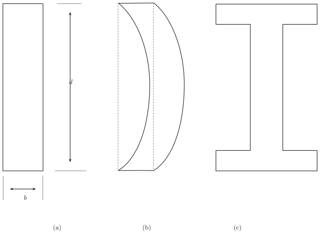
Figure 8.7 is a practical engineering sketch, not a graph. It shows three cross‑sectional shapes of a beam, each chosen to illustrate a key idea about bending and load‑bearing strength.

Panel (a) is a simple upright rectangle. The breadth $b$ is horizontal, the depth $d$ is vertical. This is the starting point: a solid rectangular bar. The important physical quantity here is the area moment of inertia (also called the second moment of area), which measures how the cross‑sectional area is distributed relative to the bending axis. For a rectangle bending about its horizontal neutral axis (the axis through its centre, parallel to $b$ ), the moment of inertia is

I = \frac{b d^{3}}{12}.

The depth $d$ appears cubed — a small increase in $d$ dramatically stiffens the beam. That is the central lesson of the figure.

Panel (b) shows what happens when the rectangle is made very thin — $d$ is small. The bar is drawn as a slender crescent, bowed sideways from its original straight outline (shown as a dashed line). This is buckling: a thin beam, when compressed along its length, does not fail by crushing but by suddenly bending sideways. The figure warns that a narrow rectangular cross‑section is unstable under compression; the beam will buckle long before the material reaches its breaking stress.

Panel (c) is the solution: an I‑beam cross‑section. It has two wide horizontal flanges (top and bottom) connected by a thin vertical web. The flanges are placed far from the neutral axis, so they contribute a large moment of inertia without adding much material. For an I‑beam, the moment of inertia is approximately

I \approx \frac{b d^{3}}{12} - \frac{(b - t_w) (d - 2t_f)^{3}}{12},

where $t_f$ is the flange thickness and $t_w$ is the web thickness. The exact formula is not needed in NCERT; the point is that $I$ is nearly as large as that of a solid rectangle of the same overall depth $d$ , but the beam is much lighter.

Important

The figure teaches one core idea: for a given amount of material, the bending stiffness is maximised by placing as much of the material as possible far from the neutral axis. That is why I‑beams, not solid rectangles, are used in bridges and buildings.

The textbook develops this figure in the context of elastic behaviour of materials — specifically, the relation between bending moment $M$ , Young’s modulus $Y$ , the moment of inertia $I$ , and the radius of curvature $R$ of the bent beam:

$\frac{M}{I} = \frac{Y}{R}.$ …

Figure 8.8Pillars or columns: (a) a pillar with rounded ends, (b) Pillar with distributed ends.

Fig. 8.8 — Pillars or columns: (a) a pillar with rounded ends, (b) Pillar with distributed ends.

Drawn by us to help you understand the concept clearly, and verified to make sure it's accurate. For exams, practice from your NCERT textbook's own diagram.

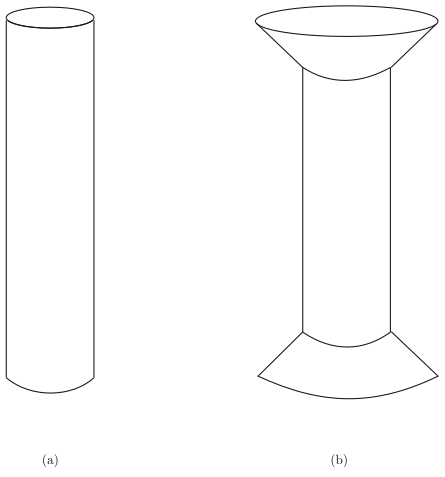
The figure contrasts two ways of designing a vertical column that must support a heavy load. On the left, panel (a) shows a simple cylindrical pillar with rounded ends — the top and bottom are smoothly curved, not flat. On the right, panel (b) shows a pillar that is narrow in the middle and flares outward at both ends into wide, flat caps. The shape in (b) is often called hourglass-like or “distributed-end” because the load from the top is spread over a larger area before it enters the column, and the reaction from the ground is similarly spread at the bottom.

The physical idea is about stress concentration. When a column has a small area of contact at its ends, the compressive stress (force per unit area) is very high at those points. Even if the column itself is strong, the material near the ends may fail first — the rounded ends in (a) still concentrate the load into a small region. By flaring the ends outward, as in (b), the same total force is distributed over a much larger area, so the stress at the ends drops dramatically. The narrow middle in (b) is not a weak point because the stress there is uniform and the column can be designed to have just enough cross-section to carry the load without wasting material.

The key formula that governs this design is the definition of compressive stress:

\sigma = \frac{F}{A}

where $\sigma$ is the stress (in pascals, Pa), $F$ is the magnitude of the compressive force (in newtons, N), and $A$ is the cross-sectional area (in m $^2$ ) at the point of interest. For a given load $F$ , the stress is inversely proportional to the area. At the ends of the column in (b), the area $A$ is large, so $\sigma$ is small. In the middle, $A$ is smaller, but the stress is still within safe limits because the column’s material can tolerate that value.

Important

The figure teaches that shape matters as much as material strength. A column with distributed ends reduces the risk of crushing at the contact surfaces, which is why real pillars in buildings and bridges often have wide capitals and bases — not just for aesthetics, but to keep the stress below the material’s ultimate compressive strength.

The textbook uses this figure in the context of applications of elastic behaviour — specifically, how engineers use the concept of stress to avoid failure. The formula for compressive strain also applies:

\epsilon = \frac{\Delta L}{L_0}

where $\epsilon$ is the strain (dimensionless), $\Delta L$ is the change in length (m), and $L_0$ is the original length (m). For a column under compression, Hooke’s law in the elastic region gives $\sigma = Y \epsilon$ , where $Y$ is Young’s modulus of the material. The distributed-end design does not change Young’s modulus, but it keeps the stress low enough that the strain remains elastic and the column does not buckle or yield. …

Start your 14-day free trial to unlock the full solution →

← Previous · 8.5.5Elastic Potential Energy in a Stretched Wire Next · summary →Summary