Physics · Ch 3 — Motion in a Plane

Addition and Subtraction of Vectors — Graphical Method

3.4

Addition and Subtraction of Vectors — Graphical Method

Why We Start with the Graphical Method

When you first learn to add vectors, the algebraic approach (using components) can feel abstract. The graphical method gives you a physical, visual feel for what vector addition actually means. You literally draw the vectors to scale and measure the result. This builds intuition before you move to the more powerful analytical methods.

The core idea is simple: vectors represent quantities that have both magnitude and direction. When you add them, you are combining these directed steps. If you walk 5 m east and then 3 m north, your total displacement is not 8 m — it is the straight-line distance from your start to your end point, in a specific direction. The graphical method captures this perfectly.

The Triangle Law of Vector Addition

This is the fundamental rule. It states:

\vec{A} + \vec{B} = \vec{R}

If two vectors $\vec{A}$ and $\vec{B}$ are represented in magnitude and direction by two sides of a triangle taken in the same order, then their resultant vector $\vec{R}$ is represented in magnitude and direction by the third side of the triangle, taken in the opposite order.

How it works, step by step:

Draw vector $\vec{A}$ to scale. Its length represents its magnitude, and its arrowhead shows its direction.
From the head (arrow tip) of $\vec{A}$ , draw vector $\vec{B}$ to the same scale, keeping its direction exactly as given.
Draw a vector from the tail (starting point) of $\vec{A}$ to the head of $\vec{B}$ . This new vector is the resultant $\vec{R}$ .

The phrase "taken in the same order" means the tail of $\vec{B}$ is placed at the head of $\vec{A}$ . The resultant then closes the triangle, going from the free tail to the free head.

Tip

The order of addition does not matter. $\vec{A} + \vec{B}$ gives the same resultant as $\vec{B} + \vec{A}$ . You can verify this by drawing $\vec{B}$ first and then $\vec{A}$ from its head. The closing side of the triangle is identical in both magnitude and direction. This is the commutative property of vector addition.

The Parallelogram Law of Vector Addition

This is an equivalent rule that is often more convenient when you have two vectors starting from the same point.

\vec{A} + \vec{B} = \vec{R}

If two vectors $\vec{A}$ and $\vec{B}$ are represented in magnitude and direction by the two adjacent sides of a parallelogram drawn from a common point, then their resultant is represented in magnitude and direction by the diagonal of the parallelogram drawn from that same common point.

How it works:

Draw vectors $\vec{A}$ and $\vec{B}$ from a common origin point O.
Complete the parallelogram. This means drawing a line parallel to $\vec{A}$ from the head of $\vec{B}$ , and a line parallel to $\vec{B}$ from the head of $\vec{A}$ .
The diagonal of the parallelogram that starts from the common origin O is the resultant $\vec{R}$ .

Note

The triangle law and the parallelogram law are not two different rules. They are two ways of looking at the same geometric construction. If you draw the triangle law, you have drawn half of the parallelogram. The diagonal of the parallelogram is exactly the same vector as the third side of the triangle.

Finding the Magnitude and Direction of the Resultant

The graphical method gives you the answer by measurement. You measure the length of $\vec{R}$ with a ruler and its angle with a protractor. But the book also derives the analytical expressions for the magnitude and direction, which are essential for later work.

Consider two vectors $\vec{A}$ and $\vec{B}$ with an angle $\theta$ between them. Let $R$ be the magnitude of the resultant $\vec{R}$ .

›Proof

Derivation of the magnitude of the resultant

Draw the parallelogram with $\vec{A}$ and $\vec{B}$ as adjacent sides. Let the common origin be O. Let $\vec{A}$ be along the x-axis for convenience.

From the head of $\vec{B}$ , drop a perpendicular to the line of $\vec{A}$ (extended if necessary). Let this foot be N. The head of $\vec{R}$ is at the point P, which is the opposite corner of the parallelogram.

In the right triangle ONP:

ON = OA + AN = $A + B \cos\theta$
NP = $B \sin\theta$

By the Pythagorean theorem:

$OP^2 = ON^2 + NP^2$

$R^2 = (A + B \cos\theta)^2 + (B \sin\theta)^2$

$R^2 = A^2 + 2AB \cos\theta + B^2 \cos^2\theta + B^2 \sin^2\theta$

$R^2 = A^2 + 2AB \cos\theta + B^2 (\cos^2\theta + \sin^2\theta)$

Since $\cos^2\theta + \sin^2\theta = 1$ :

$R^2 = A^2 + B^2 + 2AB \cos\theta$

Therefore, the magnitude of the resultant is:

$R = \sqrt{A^2 + B^2 + 2AB \cos\theta}$

›Proof

Derivation of the direction of the resultant

Let $\phi$ be the angle that the resultant $\vec{R}$ makes with $\vec{A}$ .

From the same right triangle ONP:

$\tan\phi = \frac{NP}{ON} = \frac{B \sin\theta}{A + B \cos\theta}$

Therefore, the direction of the resultant is given by:

$\phi = \tan^{-1}\left(\frac{B \sin\theta}{A + B \cos\theta}\right)$

These two formulas are the complete analytical solution for the addition of two vectors.

Watch out

The formula $R = \sqrt{A^2 + B^2 + 2AB \cos\theta}$ is valid for any angle $\theta$ between $0^\circ$ and $180^\circ$ . Do not confuse it with the Pythagorean theorem, which is only a special case when $\theta = 90^\circ$ (giving $R = \sqrt{A^2 + B^2}$ ).

Special Cases of Vector Addition

The general formula gives different results depending on the angle between the vectors.

Angle $\theta$	$\cos\theta$	Resultant Magnitude $R$	Direction $\phi$	Physical Meaning
$0^\circ$	1	$R = A + B$	$\phi = 0^\circ$	Vectors are parallel and in the same direction. The resultant is the sum of their magnitudes.
$90^\circ$	0	$R = \sqrt{A^2 + B^2}$	$\phi = \tan^{-1}(B/A)$	Vectors are perpendicular. The resultant is the hypotenuse of a right triangle.
$180^\circ$	-1	$R = \\|A - B\\|$	$\phi = 0^\circ$ if $A > B$ , $180^\circ$ if $B > A$	Vectors are antiparallel (opposite directions). The resultant is the difference of their magnitudes, in the direction of the larger vector.

Important

The magnitude of the resultant $R$ is always between the two extremes: $|A - B| \leq R \leq A + B$ . It can never be greater than the sum or less than the absolute difference of the individual magnitudes.

Subtraction of Vectors

Subtraction is defined as addition of the negative of a vector.

\vec{A} - \vec{B} = \vec{A} + (-\vec{B})

The vector $-\vec{B}$ has the same magnitude as $\vec{B}$ but points in the opposite direction. To subtract $\vec{B}$ from $\vec{A}$ graphically:

Draw vector $\vec{A}$ .
From the head of $\vec{A}$ , draw the vector $-\vec{B}$ (same length as $\vec{B}$ , but arrow pointing opposite to $\vec{B}$ 's original direction).
The resultant $\vec{R} = \vec{A} - \vec{B}$ is the vector from the tail of $\vec{A}$ to the head of $-\vec{B}$ .

Alternatively, using the parallelogram law, you can draw $\vec{A}$ and $-\vec{B}$ from a common point and draw the diagonal.

Note

The magnitude of $\vec{A} - \vec{B}$ is given by the same formula as addition, but with $\theta$ replaced by the angle between $\vec{A}$ and $-\vec{B}$ . If the angle between $\vec{A}$ and $\vec{B}$ is $\theta$ , then the angle between $\vec{A}$ and $-\vec{B}$ is $180^\circ - \theta$ . Since $\cos(180^\circ - \theta) = -\cos\theta$ , the magnitude becomes:

$|\vec{A} - \vec{B}| = \sqrt{A^2 + B^2 - 2AB \cos\theta}$

Properties of Vector Addition …

Figure 3.4(a) A and B. (b) A+B graphically. (c) B+A graphically. (d) associative law.

Fig. 3.4 — (a) A and B. (b) A+B graphically. (c) B+A graphically. (d) associative law.

Drawn by us to help you understand the concept clearly, and verified to make sure it's accurate. For exams, practice from your NCERT textbook's own diagram.

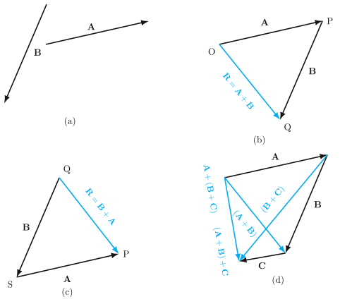
Figure 3.4 is the visual foundation for the entire idea of vector addition. It does not show a graph with axes or curves; it shows four separate panels of arrows, each panel teaching one key property of how vectors combine.

Panel (a) shows two separate arrows, labelled A and B. Each arrow has a length (representing magnitude) and a direction. At this stage they are just two independent vectors, waiting to be added.

Panel (b) is the core demonstration. Vector B is drawn starting exactly from the head (tip) of vector A. The tail of A is at point O, the head of A is at point P, and the head of B is at point Q. The resultant vector R is then drawn from the tail of A (point O) straight to the head of B (point Q). This is the head-to-tail method: you place vectors tip-to-tail in sequence, and the resultant is the single arrow that closes the triangle. The formula here is:

\mathbf{R} = \mathbf{A} + \mathbf{B}

where $\mathbf{R}$ is the vector sum, $\mathbf{A}$ is the first vector, and $\mathbf{B}$ is the second vector placed after it.

Panel (c) reverses the order. Now vector A is drawn starting from the head of vector B. The tail of B is at point S, its head at point P, and the head of A is at point Q. The resultant R is again drawn from the tail of B (point S) to the head of A (point Q). The triangle formed is different in orientation, but the resultant arrow is identical in length and direction to the one in panel (b). This demonstrates the commutative law of vector addition:

\mathbf{A} + \mathbf{B} = \mathbf{B} + \mathbf{A}

The order of addition does not change the final vector.

Panel (d) extends the idea to three vectors. It shows a quadrilateral (a four-sided shape) formed by placing vectors A, B, and C head-to-tail in sequence. The resultant R is the arrow that closes the shape from the first tail to the last head. The key lesson here is the associative law:

(\mathbf{A} + \mathbf{B}) + \mathbf{C} = \mathbf{A} + (\mathbf{B} + \mathbf{C})

Important

The figure teaches that vector addition is both commutative and associative. You can add vectors in any order, and you can group them in any way — the resultant is always the same single vector that connects the starting point to the final point. …

Figure 3.5(a) A and B, –B shown. (b) Subtracting B from A gives R2; addition R1 also shown.

Fig. 3.5 — (a) A and B, –B shown. (b) Subtracting B from A gives R2; addition R1 also shown.

Drawn by us to help you understand the concept clearly, and verified to make sure it's accurate. For exams, practice from your NCERT textbook's own diagram.

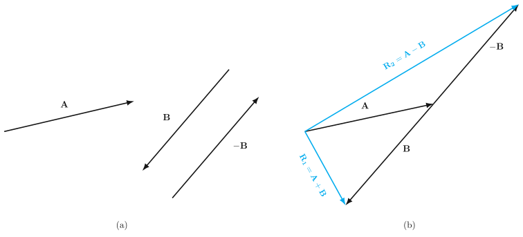
Figure 3.5 is a two-panel vector diagram that makes the idea of vector subtraction visual. In panel (a) you see three arrows drawn from a common point: vector A, vector B, and the vector –B (which is B reversed — same length, opposite direction). This panel simply establishes the two vectors you will work with and shows what the negative of B looks like. There are no axes or grid lines; the arrows are free vectors, so only their relative directions and lengths matter.

Panel (b) shows the result of combining these vectors. From the same origin, two resultant vectors are drawn. One is R₁ = A + B, the ordinary vector sum, which runs as a lower diagonal arrow. The other is R₂ = A – B, which runs as an upper diagonal arrow. Both resultants start at the tail of A and end at the head of the last vector in the chain — but the key point is that R₂ is obtained by adding A and –B using the same head-to-tail rule you use for addition. In other words, subtraction is just addition of the negative vector.

Important

Vector subtraction is not a separate operation. To subtract B from A, you reverse B to get –B and then add it to A using the triangle law of addition.

The central formula the textbook develops from this figure is the definition of vector subtraction:

\mathbf{R}_2 = \mathbf{A} - \mathbf{B} = \mathbf{A} + (-\mathbf{B})

Here, A and B are any two vectors. –B is the vector with the same magnitude as B but opposite direction. The resultant R₂ is the vector from the tail of A to the head of –B when –B is placed with its tail at the head of A. The figure also shows R₁ = A + B for comparison, so you can see that R₁ and R₂ are generally different in both magnitude and direction — subtraction is not the same as addition.

Watch out

A common mistake is to think that A – B means drawing A and then drawing B backwards from the head of A. That is exactly what you do, but the resultant is the vector from the tail of A to the head of –B, not from the tail of A to the tail of B. The figure makes this clear by showing both resultants from the same origin. …

Figure 3.6(a) Two vectors A and B with their tails brought to a common origin O. (b) The sum A+B obtained using the parallelogram method (R is the diagonal O→S). (c) The same parallelogram method shown to be equivalent to the triangle method (A then B head-to-tail from O to P to S, with the same resultant R).

Fig. 3.6 — (a) Two vectors A and B with their tails brought to a common origin O. (b) The sum A+B obtained using the parallelogram method (R is the diagonal O→S). (c) The same parallelogram method shown to be equivalent to the triangle method (A then B head-to-tail from O to P to S, with the same resultant R).

Drawn by us to help you understand the concept clearly, and verified to make sure it's accurate. For exams, practice from your NCERT textbook's own diagram.

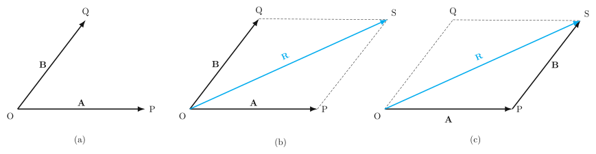
Figure 3.6 is the visual foundation for how vectors add. It shows three panels that build from two separate vectors to the idea that vector addition is equivalent whether you complete a parallelogram or form a triangle.

Panel (a) is the starting point. Two vectors, A and B, are drawn with their tails together at a common origin O. A goes from O to point P, and B goes from O to point Q. The only thing shown here is the two vectors in their natural positions, ready to be combined.

Panel (b) introduces the parallelogram rule. From the tip of A (point P), a dashed line is drawn parallel to B. From the tip of B (point Q), a dashed line is drawn parallel to A. These two dashed lines meet at a new point S, completing the parallelogram OPSQ. The diagonal of this parallelogram, from the common origin O to the opposite vertex S, is the resultant vector R. This is the vector sum A + B. The physical idea is that if you walk along A and then along B, you end up at the same place as if you had walked along the diagonal R — but the diagonal path is a straight line, not a turn.

Panel (c) shows the same addition, but now as a triangle. Vector B is redrawn so its tail sits at the tip of A (point P), and its tip now lands at S. The vector from O to S is still R. This is the triangle method: place the tail of the second vector at the head of the first, and the resultant runs from the tail of the first to the head of the second. The figure’s caption explicitly says “parallelogram ≡ triangle method” — they are exactly equivalent. The parallelogram just shows both vectors starting from the same point; the triangle shows them head-to-tail.

Important

The key result from this figure is the vector addition formula. For two vectors A and B with an angle $\theta$ between them, the magnitude of the resultant R is given by the law of cosines applied to the triangle OPS:

R = \sqrt{A^2 + B^2 + 2AB\cos\theta}

Here $A$ and $B$ are the magnitudes of the vectors, and $\theta$ is the angle between them when placed tail-to-tail. The direction of R is given by the angle $\phi$ it makes with A:

\tan\phi = \frac{B\sin\theta}{A + B\cos\theta}

The figure itself does not show these formulas — it only shows the geometry. But the geometry is the proof. In the triangle OPS (panel c), side OP is $A$ , side PS is $B$ , and the angle at O between A and B is $\theta$ . The side OS is $R$ , and by the law of cosines, $R^2 = A^2 + B^2 - 2AB\cos(\pi - \theta)$ . Since $\cos(\pi - \theta) = -\cos\theta$ , this becomes $R^2 = A^2 + B^2 + 2AB\cos\theta$ . …

Start your 14-day free trial to unlock the full solution →

← Previous · 3.3Multiplication of Vectors by Real Numbers Next · 3.4 →Example 3.1 — Rain is falling vertically with a speed of 35m s⁻¹. Winds starts blowi…