Physics · Ch 2 — Motion in a Straight Line

Acceleration

2.3

Acceleration

The Meaning of Acceleration

When an object’s velocity changes — either in magnitude, direction, or both — we say it is accelerating. In straight-line motion, direction is fixed, so acceleration is simply the rate at which the velocity changes with time.

If a car’s speedometer reading goes from 20 km/h to 40 km/h in 5 seconds, its velocity is increasing. If it goes from 40 km/h to 20 km/h in the same time, its velocity is decreasing — that is also acceleration, but in the opposite direction (often called deceleration or retardation).

Note

In physics, “acceleration” always means any change in velocity, not just speeding up. Slowing down is acceleration with a negative sign relative to the direction of motion.

Average Acceleration

Average acceleration is defined as the change in velocity divided by the time interval over which that change occurs.

If at time $t_1$ the velocity is $v_1$ , and at time $t_2$ the velocity is $v_2$ , then the average acceleration $\bar{a}$ over the interval $\Delta t = t_2 - t_1$ is:

\bar{a} = \frac{v_2 - v_1}{t_2 - t_1} = \frac{\Delta v}{\Delta t}

The SI unit of acceleration is metre per second squared, written as $\text{m s}^{-2}$ . In everyday life, we might use $\text{km h}^{-2}$ or $\text{cm s}^{-2}$ , but in physics problems, stick to $\text{m s}^{-2}$ .

Watch out

A common mistake is to think that if velocity is zero, acceleration must also be zero. Not true. At the highest point of a ball thrown upward, velocity is zero for an instant, but acceleration due to gravity is still $9.8\ \text{m s}^{-2}$ downward. Zero velocity does not imply zero acceleration.

Instantaneous Acceleration

Average acceleration tells us the overall change over a finite interval. But velocity can change in a complicated way — it might be increasing rapidly at one moment and slowly the next. To know the acceleration at a specific instant, we take the limit of the average acceleration as the time interval approaches zero.

Instantaneous acceleration $a$ is:

a = \lim_{\Delta t \to 0} \frac{\Delta v}{\Delta t} = \frac{dv}{dt}

Since velocity itself is $v = dx/dt$ , acceleration is the second derivative of position with respect to time:

a = \frac{dv}{dt} = \frac{d}{dt}\left(\frac{dx}{dt}\right) = \frac{d^2 x}{dt^2}

Important

Acceleration is the slope of the velocity–time graph at any instant. If the $v$ – $t$ graph is a straight line, the slope is constant and acceleration is uniform. If the graph is curved, the slope changes from point to point, and acceleration varies with time.

Properties of Acceleration in Straight-Line Motion

The textbook lists three key properties that follow directly from the definition $a = dv/dt$ . Each one is proved below.

›Proof

Property (I): If the velocity of an object is constant, its acceleration is zero.

If $v = \text{constant}$ , then $dv/dt = 0$ . Therefore $a = 0$ .

Property (II): If the velocity of an object is increasing with time, its acceleration is positive.

“Increasing with time” means $dv/dt > 0$ . Hence $a > 0$ .

Property (III): If the velocity of an object is decreasing with time, its acceleration is negative.

“Decreasing with time” means $dv/dt < 0$ . Hence $a < 0$ .

These properties are straightforward, but they depend on the chosen direction. If you define the positive direction as east, then a car speeding up while moving east has positive acceleration. The same car speeding up while moving west has negative velocity but also negative acceleration (since its velocity is becoming more negative). The sign of acceleration tells you whether the velocity is becoming more positive or more negative. …

Figure 2.2Position-time graph for motion with (a) positive acceleration; (b) negative acceleration, and (c) zero acceleration.

Fig. 2.2 — Position-time graph for motion with (a) positive acceleration; (b) negative acceleration, and (c) zero acceleration.

Drawn by us to help you understand the concept clearly, and verified to make sure it's accurate. For exams, practice from your NCERT textbook's own diagram.

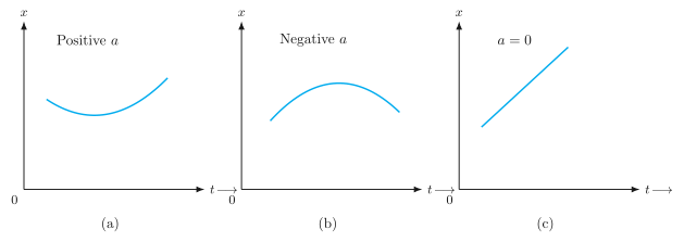
The figure shows three position–time graphs side by side, each with the vertical axis labelled $x$ (position) and the horizontal axis labelled $t$ (time), both meeting at the origin. The three panels illustrate how the shape of the $x$ – $t$ curve changes when acceleration is positive, negative, or zero.

In panel (a), the curve rises and bends upward — it is concave up. This shape tells you that the slope (which is velocity) is increasing as time passes. A car starting from rest and speeding up would produce such a graph: the position changes slowly at first, then more and more rapidly. The physical idea is that positive acceleration means velocity is increasing with time, so the $x$ – $t$ graph curves away from the time axis.

Panel (b) shows a curve that rises to a peak and then falls — a dome shape that is concave down. Here the slope starts positive, decreases to zero at the top, then becomes negative. This corresponds to negative acceleration (or deceleration): the velocity is decreasing. Think of a ball thrown upward: it slows down as it rises, stops momentarily at the highest point, then speeds up downward. The graph’s curvature tells you the velocity is becoming less positive (or more negative) over time.

Panel (c) is a straight line sloping upward from the origin. A straight line means the slope is constant — velocity does not change. That is zero acceleration: uniform motion at constant speed. The position increases by equal amounts in equal time intervals.

Important

The key lesson from these three curves is that acceleration is the curvature of the position–time graph. Concave up means positive acceleration, concave down means negative acceleration, and a straight line means zero acceleration.

The textbook develops the definition of acceleration directly from this figure. If $v$ is the velocity at time $t$ , then average acceleration $\bar{a}$ over a time interval $\Delta t$ is

\bar{a} = \frac{\Delta v}{\Delta t}

and instantaneous acceleration is the limit

a = \lim_{\Delta t \to 0} \frac{\Delta v}{\Delta t} = \frac{dv}{dt}

Since velocity itself is $v = dx/dt$ , acceleration is the second derivative of position:

a = \frac{d^2 x}{dt^2}

Each symbol: $x$ is position (in metres), $t$ is time (in seconds), $v$ is velocity (m/s), $a$ is acceleration (m/s²). The figure makes this abstract idea concrete: the slope of the $x$ – $t$ graph gives $v$ , and the rate at which that slope changes — the curvature — gives $a$ . …

Figure 2.3Velocity-time graph for motions with constant acceleration. (a) Motion in positive direction with positive acceleration, (b) Motion in positive direction with negative acceleration, (c) Motion in negative direction with negative acceleration, (d) Motion of an object with negative acceleration that changes direction at time t1.

Fig. 2.3 — Velocity-time graph for motions with constant acceleration. (a) Motion in positive direction with positive acceleration, (b) Motion in positive direction with negative acceleration, (c) Motion in negative direction with negative acceleration, (d) Motion of an object with negative acceleration that changes direction at time t1.

Drawn by us to help you understand the concept clearly, and verified to make sure it's accurate. For exams, practice from your NCERT textbook's own diagram.

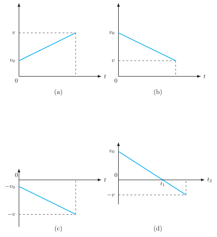
The four panels of Fig. 2.3 are a single lesson: the slope of a velocity–time graph is the acceleration, and that slope can be positive, negative, or zero regardless of whether the velocity itself is positive or negative. Each panel is a straight line, meaning the acceleration is constant in every case.

Panel (a) shows a line that starts at $v_0$ on the velocity axis and rises steadily to $v$ at a later time. Both $v_0$ and $v$ are positive numbers, and the line slopes upward. The slope is positive, so the acceleration $a$ is positive. The object moves in the positive direction (velocity positive) and speeds up.

Panel (b) also begins at a positive $v_0$ , but the line falls to a smaller positive $v$ . The slope is negative, so $a$ is negative. The object still moves in the positive direction, but it slows down — this is deceleration in the everyday sense.

Panel (c) is the mirror of (a) in the negative region. The line starts at $-v_0$ (negative velocity) and goes down to $-v$ , which is even more negative. The slope is negative, so $a$ is negative. The object moves in the negative direction and its speed (magnitude of velocity) increases.

Panel (d) is the most instructive. The line begins at a positive $v_0$ , crosses the time axis at $t_1$ (where $v=0$ ), and continues into the negative region to $-v$ at $t_2$ . The slope is negative throughout — the acceleration is constant and negative. At $t_1$ the object momentarily stops, then reverses direction and moves in the negative direction, gaining speed in that direction. This single graph captures a complete reversal of motion under constant acceleration.

Watch out

A common mistake is to think that a negative slope always means "slowing down." Panel (c) shows that a negative slope can mean speeding up in the negative direction. What matters is the sign of the acceleration relative to the sign of the velocity: when they have the same sign, speed increases; when opposite, speed decreases.

The key formula that emerges from these straight-line graphs is the first equation of motion for constant acceleration. For any straight line on a $v$ – $t$ graph, the slope is

a = \frac{v - v_0}{t}

which rearranges to

v = v_0 + a t

where $v_0$ is the velocity at $t=0$ , $v$ is the velocity at time $t$ , and $a$ is the constant acceleration. This formula works for all four panels: plug in the appropriate signs for $v_0$ , $v$ , and $a$ , and it correctly describes the line.

v = v_0 + a t

Figure 2.4Area under v-t curve equals displacement of the object over a given time interval.

Fig. 2.4 — Area under v-t curve equals displacement of the object over a given time interval.

Drawn by us to help you understand the concept clearly, and verified to make sure it's accurate. For exams, practice from your NCERT textbook's own diagram.

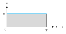
The figure shows a velocity–time graph for the simplest possible motion: an object moving with constant velocity $u$ . The horizontal axis is time $t$ , measured from $0$ to $T$ . The vertical axis is velocity $v$ . Because the velocity never changes, the graph is a straight horizontal line at height $u$ above the time axis, running from $t = 0$ to $t = T$ .

The shaded region under this line is a rectangle. Its base is the time interval $T$ (from $0$ to $T$ ), and its height is the constant velocity $u$ . The area of that rectangle is $u \times T$ .

What does that area represent? For motion at constant velocity, displacement is simply velocity multiplied by time:

\text{displacement} = u \times T

That is exactly the area of the shaded rectangle. So the figure makes a powerful geometric point: the area enclosed between the velocity–time curve and the time axis, over a given interval, equals the displacement of the object during that interval.

Important

This is not a coincidence for constant velocity — it is a general result. For any velocity–time graph, the area under the curve (taking sign into account) gives the displacement. The constant-velocity case is the simplest illustration: the curve is a flat line, so the area is just a rectangle.

The key formula the textbook develops from this figure is therefore:

\text{Displacement} = \text{Area under } v(t) \text{ curve from } t_1 \text{ to } t_2

For the specific case shown, with $v(t) = u$ (constant) from $t = 0$ to $t = T$ :

s = u \times T

where $s$ is the displacement, $u$ is the constant velocity, and $T$ is the time interval. Every symbol is defined directly from the axes of the graph: $u$ is the height of the horizontal line (the velocity), $T$ is the length of the base (the time elapsed), and their product is the area of the shaded rectangle — which is the displacement. …

Start your 14-day free trial to unlock the full solution →

← Previous · 2.2Example 2.1 — The position of an object moving along x-axis is given by x = a + bt² …Next · 2.4 →Kinematic Equations for Uniformly Accelerated Motion