(a) You are given the consumption function of an imaginary economy, C = 100 + 0·8 Y, where C = Consumption and

Question 36 of 104

Q. (a) You are given the consumption function of an imaginary economy, C = 100 + 0\cdot8 Y, where C = Consumption and Y = Income. Calculate :

(i) The value of Marginal Propensity to Save (MPS)

(ii) The level of income at Break-Even Point

(OR)

(b) S = − 60 + 0·1 Y is the saving function, where S is Saving and Y is National Income and Investment Expenditure (I) is ₹ 4,000 crore in an economy. Calculate the Equilibrium level of Income.

CBSECBSE Class XII Board 2022Subjective· 2mImportance★★★★★

35% · 36/104 Questions

🔒 Locked · start free trial →

You're viewing a preview — the full solution, concept, methods & PYQ mapping are locked.

Start your 14-day free trial to unlock the full solution →

Concept understanding — Marginal Propensity to Consume

Marginal Propensity to Consume (MPC)

Start with everyday intuition

Think about what happens when you get some extra money — say, a ₹500 bonus from your part-time job, or a cash gift on your birthday. You don't save all of it, and you don't spend all of it either. Most people spend a part and save the rest. That part you spend — the fraction of the extra income that goes into consumption — is exactly what economists call the Marginal Propensity to Consume.

The word "marginal" here means "extra" or "additional." So MPC answers one simple question: Out of every extra rupee you earn, how much do you spend?

The precise meaning

Formally, MPC is the ratio of change in consumption expenditure to the change in income that brought it about.

MPC = \frac{\Delta C}{\Delta Y}

For example, if your income rises by ₹1,000 and your consumption rises by ₹750, your MPC is $750/1000 = 0.75$ (or 75%). This means you spend 75 paise of every extra rupee and save the remaining 25 paise.

The other side of the coin is the Marginal Propensity to Save (MPS) — the fraction of extra income that is saved. Since every extra rupee is either spent or saved:

MPC + MPS = 1

This is not a theory; it's an accounting identity. If MPC = 0.75, then MPS must be 0.25.

Why MPC matters

MPC is not just a number — it is the engine of the multiplier effect, one of the most powerful ideas in macroeconomics.

When someone spends money, that spending becomes someone else's income. That second person, in turn, spends a fraction (their MPC) of that income, which becomes a third person's income, and so on. A single initial injection of spending — say, government investment in a road — ripples through the economy, generating total income many times larger than the original spending.

The size of this ripple depends directly on MPC. The higher the MPC, the larger the multiplier.

Multiplier\ (k) = \frac{1}{1 - MPC} = \frac{1}{MPS}

If MPC = 0.8, the multiplier is $1/(1-0.8) = 5$ . An initial ₹100 crore investment can generate ₹500 crore of total income. If MPC = 0.5, the multiplier is only 2.

A word on the diagram …

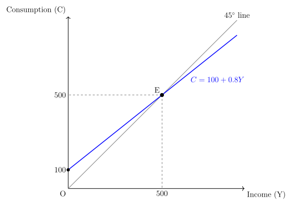
Part (a): from $C = 100 + 0.8Y$ , MPS = 1 − 0.8 = 0.2 and the break-even income (where $Y = C$ ) is ₹500. Part (b): from $S = -60 + 0.1Y$ with $I = ₹4,000$ crore, equilibrium income (where $S = I$ ) is ₹40,600 crore.

Consumption function $C = 100 + 0.8Y$

The slope of the consumption function is the MPC = 0.8; the intercept 100 is autonomous consumption.

Marginal Propensity to Save. Since $\text{MPC} + \text{MPS} = 1$ : $\text{MPS} = 1 - 0.8 = 0.2$
Break-even level of income. The break-even point is where income is entirely consumed, i.e. $C = Y$ (saving = 0): $Y = 100 + 0.8Y \Rightarrow Y - 0.8Y = 100 \Rightarrow 0.2Y = 100 \Rightarrow Y = \frac{100}{0.2} = 500$
Note

The break-even point (saving = 0) is not the same as the equilibrium income (planned saving = planned investment).

Start your 14-day free trial to see the full solution →

Concept understanding — Aggregate Demand Equilibrium

Aggregate Demand Equilibrium: The Economy's Balancing Act

Think of a seesaw. On one side sits everything people, firms, and the government want to buy. On the other side sits everything firms produce. When the seesaw is perfectly level — when total spending exactly matches total output — the economy is in equilibrium. That's the core idea.

But why should you care? Because when the seesaw tilts, real things happen. If spending exceeds output, prices rise (inflation). If output exceeds spending, factories shut down and people lose jobs. Equilibrium is the sweet spot where neither happens.

The Precise Meaning

In macroeconomics, Aggregate Demand (AD) is the total planned spending on final goods and services in an economy during a given period. Aggregate Supply (AS) is the total output firms plan to produce.

Equilibrium occurs where:

AD = AS

At this point, what buyers intend to spend exactly equals what sellers intend to produce. No unwanted inventories pile up, and no shortages force prices up. The economy is "at rest."

Y = C + I + G + (X - M)

This is the AD identity from your NCERT textbook. It tells you that total spending in the economy comes from four sources: households, firms, government, and foreigners (net of what we buy from them).

How Equilibrium Actually Works

Imagine a simple economy with only households and firms. Households earn income $Y$ from firms. They spend part of it on consumption $C$ and save the rest $S$ . Firms produce output and also invest $I$ (buying machines, building factories).

Equilibrium condition becomes:

Y = C + I

But households don't spend all their income. They save. So $C = Y - S$ . Substituting:

Y = (Y - S) + I

Which simplifies to:

S = I

Important

In equilibrium, planned savings must equal planned investment. This is the Keynesian cross condition. If people save more than firms invest, total spending falls short of output — inventories pile up, firms cut production, and income falls until savings and investment match again.

The 45° Line Diagram (Describe It)

Draw a graph with Aggregate Demand (AD) on the vertical axis and National Income (Y) on the horizontal axis.

Draw a 45° line from the origin. Every point on this line represents $AD = Y$ — the equilibrium condition.
Draw the AD curve (which is $C + I + G + (X-M)$ ). It slopes upward because as income rises, consumption rises.
Where the AD curve crosses the 45° line — that's the equilibrium point. …

Part (b) — Saving function $S = -60 + 0.1Y$ , $I = ₹4,000$ crore …

Start your 14-day free trial to see the full solution →

Same / Similar Concept — real previous-year questions on the same or a closely similar concept, not this exact question.

Showing the 12 most recent of 158 on this concept.

CBSE 2026Set 58/1/11 markMCQ
$Q. In an economy, when __________ is insufficient to achieve the level of output corresponding to the full employment, the difference is termed a deflationary gap. (Choose the correct option to fill in the blank) Options : (A) ex-ante Aggregate Demand (B) ex-post Aggregate Demand (C) ex-ante Aggregate Supply (D) ex-post Aggregate Supply$
›Reveal solutionSolution

A deflationary gap occurs when planned (ex-ante) aggregate demand falls short of the level needed for full-employment output. The correct answer is (A) ex-ante Aggregate Demand.

Let’s first get the concept clear. In macroeconomics, the term “gap” refers to the difference between what the economy is actually producing and what it could produce if all resources (labour, capital) were fully employed. That full-employment level of output is also called potential output.

Now, what determines actual output in the short run? According to the Keynesian framework, it is aggregate demand that drives production. Firms produce only as much as they expect to sell. So if total planned spending in the economy — what buyers intend to buy — is less than the value of full-employment output, firms will not produce that full-employment output. They will produce less, leading to unemployment and idle capacity.

That shortfall in planned spending is the deflationary gap. The word “deflationary” signals that the pressure on prices is downward — because demand is too weak to absorb all that could be produced.

Now, why must it be ex-ante (planned) and not ex-post (actual)? Ex-post aggregate demand is always equal to actual output by definition (because what is produced is what is sold, once you account for inventory changes). So ex-post demand can never be “insufficient” — it always matches whatever output happens to be. The gap is about intentions not matching the full-employment target. That is why we use ex-ante concepts.
$Deflationary gap = Full-employment output - Actual output (where actual output is determined by ex-ante aggregate demand) \dots$
Start your 14-day free trial to see the full solution →
CBSE 2026Set 58/1/11 markMCQ
$Q. Identify, which of the following is true at the Break Even level of Income. (Choose the correct option) Options : (A) Slope of Consumption Curve = Slope of Saving Curve (B) Average Propensity to Consume (APC) = Average Propensity to Save (APS) (C) Slope of Saving Curve = Unity$
(1) (D) Average Propensity to Consume (APC) = Unity (1)
›Reveal solutionSolution

At break-even income, consumption exactly equals income (saving is zero), which means the entire income is consumed — so APC = 1.

The break-even point in consumption theory is the level of income at which a household or economy consumes exactly what it earns. There is no saving and no dissaving; the consumption function intersects the 45° line (where $C = Y$ ).

To see which statement holds at this point, recall what break-even means algebraically. If income is $Y$ and consumption is $C$ , then at break-even:
$C = Y$
Since saving $S = Y - C$ , we have:
$S = Y - Y = 0$
Now examine each option in turn.

Option (A): Slope of Consumption Curve = Slope of Saving Curve

The slope of the consumption curve is the marginal propensity to consume, $\text{MPC} = \frac{dC}{dY}$ . The slope of the saving curve is the marginal propensity to save, $\text{MPS} = \frac{dS}{dY}$ . We know that $\text{MPC} + \text{MPS} = 1$ always (since any additional rupee of income is either consumed or saved), so $\text{MPC} = \text{MPS}$ would require both to equal $0.5$ . This is not a general property of the break-even point — it depends on the specific consumption function. The break-even condition tells us nothing about the slopes.

Option (B): Average Propensity to Consume (APC) = Average Propensity to Save (APS)

The average propensity to consume is $\text{APC} = \frac{C}{Y}$ and the average propensity to save is $\text{APS} = \frac{S}{Y}$ . At break-even, $C = Y$ and $S = 0$ , so:
$\text{APC} = \frac{Y}{Y} = 1, \quad \text{APS} = \frac{0}{Y} = 0$
These are not equal.

Option (C): Slope of Saving Curve = Unity (1) …
Start your 14-day free trial to see the full solution →
CBSE 2026Set 58/2/11 markMCQ
$Q. Choose the correct consumption function from the options given below with reference to the illustrated given diagram. (Diagram: X-axis = Income, Y-axis = Consumption; a 45° Income Line; a consumption curve C with a positive intercept of 100; equilibrium point E where the C curve cuts the 45° line; dashed lines mark C = 280 at one income level and C = 700 at income = 800.) Options : (A) C = 100 + 0.7Y (B) C = 100 + 0.8Y (C) C = 100 - 0.7Y (D) C = 100 - 0.8Y$
›Reveal solutionSolution

The consumption curve has autonomous consumption $\bar{C}=100$ (its vertical intercept) and its slope is the MPC. Using the break-even point $E$ where the curve cuts the $45°$ line ( $C=Y=500$ ), the MPC works out to exactly $0.8$ , so the consumption function is $C = 100 + 0.8Y$ — option (B).

The consumption function and its components

A consumption function describes the relationship between national income $Y$ and aggregate consumption $C$ . The standard Keynesian form is
$C = \bar{C} + c \, Y$
where $\bar{C}$ is autonomous consumption (consumption when income is zero — the vertical intercept) and $c$ is the marginal propensity to consume (MPC), the fraction of each additional rupee of income spent on consumption, and geometrically the slope of the line.

The diagram gives us two facts. First, the consumption curve has a positive vertical intercept of $100$ , so $\bar{C} = 100$ . Second, the curve is upward-sloping, which immediately rules out options (C) and (D): a negative coefficient would mean consumption falls as income rises, contradicting both theory and the diagram.

Finding the MPC from the break-even point

The cleanest way to read the slope off this diagram is the break-even point $E$ , where the consumption curve intersects the $45°$ line. Along the $45°$ line every point satisfies $C = Y$ , so at $E$ consumption exactly equals income. From the diagram, this occurs at $Y = C = 500$ .

Substituting $\bar{C} = 100$ and the point $(Y, C) = (500, 500)$ into $C = \bar{C} + cY$ :
$500 = 100 + c(500)$ $400 = 500c$
$c = \frac{400}{500} = 0.8$ …
Start your 14-day free trial to see the full solution →
CBSE 2026Set 58/2/11 markMCQ
$Q. The Aggregate Demand (AD) curve lies parallel to consumption curve, indicating that both have ________. (Choose the correct option to fill in the blank) (A) same components (B) different slope (C) same slope (D) inverse relationship$
›Reveal solutionSolution
The Aggregate Demand (AD) curve is derived by vertically shifting the consumption curve upwards by the amount of autonomous expenditures; since these additions are independent of income, the slope of the AD curve remains the same as the slope of the consumption curve, which is the Marginal Propensity to Consume (MPC).

To understand why the Aggregate Demand (AD) curve lies parallel to the consumption curve, we need to examine the components and slopes of both.

First, let's consider the consumption function. In Keynesian economics, the consumption function describes the relationship between consumption expenditure and disposable income. It is typically represented as:

$C = \bar{C} + bY$

where:

$C$ is total consumption expenditure.

$\bar{C}$ is autonomous consumption (consumption that occurs even when income is zero).

$b$ is the Marginal Propensity to Consume (MPC), which is the change in consumption for a unit change in income ( $\Delta C / \Delta Y$ ).

$Y$ is disposable income.

The slope of the consumption curve is given by $b$ , the Marginal Propensity to Consume. This value indicates how much of an additional rupee of income is spent on consumption.

Next, let's look at the Aggregate Demand (AD) function. Aggregate Demand represents the total demand for goods and services in an economy at a given price level. In a simple two-sector economy (households and firms), AD is the sum of consumption (C) and investment (I):

$AD = C + I$

Substituting the consumption function into the AD equation:

$AD = (\bar{C} + bY) + I$

In this simplified model, investment ( $I$ ) is often assumed to be autonomous, meaning it does not depend on the level of income. It is determined by factors like interest rates, business expectations, and government policy. Therefore, $I$ is a constant value.

We can rearrange the AD function as:

$AD = (\bar{C} + I) + bY$
$AD = (\bar{C} + I) + bY$
Start your 14-day free trial to see the full solution →
CBSE 2026Set 58/3/11 markMCQ
$Q. Select the correct formula to calculate the value of Marginal Propensity to Save (MPS) : I. Change in Savings (ΔS) / Change in Consumption (ΔC) II. Change in Savings (ΔS) / Change in Income (ΔY) III. 1 - Marginal Propensity to Consume (MPC) IV. Change in Income (ΔY) / Change in Savings (ΔS) Options : (A) I, II, III and IV (B) II and III (C) Only III (D) Only II$
›Reveal solutionSolution

MPS measures the fraction of additional income that households save rather than consume. The correct formulas are II (ΔS/ΔY, the definition) and III (1 – MPC, from the income identity), so the answer is (B).

The Marginal Propensity to Save captures a simple behavioral question: when your income rises by one rupee, how much of that extra rupee do you tuck away as savings? It's the savings counterpart to the Marginal Propensity to Consume.

Start with the fundamental income identity. Every rupee of additional income must be either consumed or saved—there is no third bucket. Mathematically, for any change in income:
$\Delta Y = \Delta C + \Delta S$
Divide both sides by $\Delta Y$ :
$\frac{\Delta Y}{\Delta Y} = \frac{\Delta C}{\Delta Y} + \frac{\Delta S}{\Delta Y}$ $1 = \text{MPC} + \text{MPS}$
This tells us immediately that MPS = 1 – MPC (option III is correct). If households consume 0.75 of each additional rupee, they must save the remaining 0.25; the two propensities are complementary fractions of the same whole.
$\text{MPS} = \frac{\Delta S}{\Delta Y} = 1 - \text{MPC}$
Now examine the definition. MPS is the responsiveness of savings to income, so by definition it is the ratio of the change in savings to the change in income that caused it: ΔS/ΔY (option II is correct). This is the direct, textbook definition—just as MPC is ΔC/ΔY, MPS is ΔS/ΔY. …
Start your 14-day free trial to see the full solution →
CBSE 2026Set 58/3/11 markMCQ
$Q. Suppose in a hypothetical economy, Y = 50 + 0\cdot8Y + 100, where Y = National Income. The value of Investment Multiplier (K) would be __________. (Choose the correct option to fill in the blank) Options : (A) 5 (B) 0\cdot2 (C) 50 (D) 0\cdot8$
›Reveal solutionSolution
The given equation represents the equilibrium condition for national income. By identifying the Marginal Propensity to Consume (MPC) from this equation, we can calculate the Investment Multiplier using its standard formula. The value of the Investment Multiplier is $\boxed{5}$ .

In macroeconomics, the equilibrium level of national income ( $Y$ ) is achieved when the aggregate demand (AD) in the economy equals the aggregate supply (AS), which is equivalent to the total output or national income. In a simple two-sector economy (households and firms), aggregate demand consists of consumption (C) and investment (I). Thus, the equilibrium condition is $Y = C + I$ .

The given equation, $Y = 50 + 0.8Y + 100$ , directly represents this equilibrium. Here, the term $50 + 0.8Y$ corresponds to the consumption function ( $C$ ), and $100$ represents autonomous investment ( $I$ ).

The consumption function, $C = a + bY$ , shows how consumption expenditure relates to national income. In this function:

$a$ is autonomous consumption (consumption that occurs even at zero income). Here, $a = 50$ .

$b$ is the Marginal Propensity to Consume (MPC), which indicates the proportion of an additional unit of income that is spent on consumption. Here, $b = 0.8$ .

The Investment Multiplier (K) is a crucial concept that explains how an initial change in autonomous investment leads to a much larger change in the equilibrium level of national income. It arises because an initial investment creates income, which is then partly consumed, leading to further income generation, and so on, in a continuous cycle. The size of this multiplier effect depends directly on the Marginal Propensity to Consume (MPC). A higher MPC means a larger portion of additional income is consumed, leading to a stronger multiplier effect. …
Start your 14-day free trial to see the full solution →
CBSE 2026Set 58/3/11 markMCQ
$Q. Read the following statements carefully : Statement I : At the break-even level of income, the value of slope of the consumption curve is zero. Statement II : Marginal Propensity to Consume (MPC) refers to the change in consumption per unit change in income. In the light of the given statements, choose the correct option from the following : (A) Statement I is true and Statement II is false. (B) Statement I is false and Statement II is true. (C) Both Statements I and II are true. (D) Both Statements I and II are false.$
›Reveal solutionSolution

Statement I is false because the slope of the consumption curve at break-even income is the MPC, which is positive (not zero). Statement II is true because MPC is defined as the change in consumption per unit change in income.

Let’s unpack this carefully. The question tests two distinct ideas from the theory of consumption and income determination — the break-even point and the meaning of Marginal Propensity to Consume (MPC).

Statement I talks about the break-even level of income. In macroeconomics, the break-even point is that level of income where consumption exactly equals income — so saving is zero. At this point, the consumption curve (which plots consumption against income) is not flat; it has a positive slope. Why? Because the consumption function is typically written as $C = \bar{C} + bY$ , where $\bar{C}$ is autonomous consumption (positive even at zero income) and $b$ is the MPC — the slope of the curve. At break-even, $C = Y$ , so $\bar{C} + bY = Y$ , which gives $Y = \bar{C} / (1-b)$ . The slope here is still $b$ , which is a positive fraction (between 0 and 1). It is never zero unless MPC is zero, which would mean consumption never changes with income — a situation that contradicts the basic Keynesian consumption function. So Statement I is false.

Note

A common confusion: students sometimes think “break-even” means the curve is horizontal. But break-even is about the level of income where C = Y, not about the slope. The slope remains the MPC throughout. …

Start your 14-day free trial to see the full solution →
CBSE 2026Set MARCH1 markMCQ
$Q. Rate of change in savings as income increases is$
(a) Average propensity to consume
(b) Average propensity to save
(c) Marginal propensity to save
(d) Marginal propensity to consume
›Reveal solutionSolution

The rate of change in saving as income changes is the marginal propensity to save, so the answer is (c).

…

Start your 14-day free trial to see the full solution →
CBSE 2026Set ANNUAL1 markMCQ
$Q. The consumer does not change his consumption despite change in his income, than the value of MPC will be A) MPC > 1 B) MPC = 1 C) MPC = 0 D) MPC < 1$
›Reveal solutionSolution

No change in consumption when income changes means MPC = 0, so the answer is C.

Marginal Propensity to Consume (MPC) = change in consumption (ΔC) ÷ change in income (ΔY). The question states the consumer does not change consumption despite a change in income, so ΔC = 0. Therefore MPC = 0 ÷ ΔY = 0. Values like MPC > …

Start your 14-day free trial to see the full solution →
CBSE 2026Set ANNUAL1 markMCQ
$Q. Formula of consumption function is A) C = C̄ - cY B) C = C̄ + cY C) C = S̄ - cY D) C = S̄ + cY$
›Reveal solutionSolution

The consumption function is C = C̄ + cY, so the answer is B.

In the Keynesian consumption function, C̄ is autonomous consumption (the consumption that takes place even at zero income) and c is the marginal propensity to consume, so cY is the induced consumption that rises with income Y. Consumption therefore increases with incom …

Start your 14-day free trial to see the full solution →
CBSE 2026Set ANNUAL1 mark
$Q. Fill in the blank: In two sector model, there are two sources of demand, the first is consumption and the second is ________.$
›Reveal solutionSolution

The blank is filled by 'investment'.

The two-sector model includes only households and firms (no government or foreign sector). Here aggregate demand (AD) for goods and services comes from two sources: consumption expenditure (C) by households and investment expenditure (I) by firms, so AD = C + I. Since the first source given is consumpti …

Start your 14-day free trial to see the full solution →
CBSE 2026Set ANNUAL1 mark
$Q. Define the average propensity to consume.$
›Reveal solutionSolution

APC is total consumption divided by total income: APC = C/Y.

The Average Propensity to Consume (APC) measures the proportion of total income that households spend on consumption. It is defined as APC = C ÷ Y, where C is total consumption expenditure and Y is total (disposable) income. For example, if income is ₹1,000 and consumption is ₹800, then APC = 800 ÷ 1,000 = 0.8, meaning 80% of income is consumed. This is a standard definition in the Class-12 …

Start your 14-day free trial to see the full solution →

←Previous questionQ29 — Define Inflationary Gap. State, how the government can control the sit…→Next questionQ31 — (a) If planned savings exceed planned investments in an economy, state…

Q.(a) You are given the consumption function of an imaginary economy, C = 100 + 0·8 Y, where C = Consumption and Y = Income. Calculate :