(a) "If actual demand for final goods falls short of the actual output of final goods corresponding to full employment level, it may lead to an unintended accumulation of inventories." Do you agree with the given statement? Give valid reasons in support of your answer. OR (b) Complete the following table. Construct the consumption function at ₹ 200 crore level of income. | Table columns: Income (Y) (in ₹ crore) | Savings (S) (in ₹ crore) | Average Propensity to Consume (APC) | Marginal Propensity to Save (MPS) | | --- | --- | --- | --- | | Rows: 0 | (–) 50 | – | – ; | | 100 | ........ | 1 | ........ ; | | 200 | ........ | 3/4 | ........ ; | | 300 | ........ | 2/3 | ........ |

(a) "If actual demand for final goods falls short of the actual output of final goods corresponding to full em

Question 70 of 104

"If actual demand for final goods falls short of the actual output of final goods corresponding to full employment level, it may lead to an unintended accumulation of inventories." Do you agree with the given statement? Give valid reasons in support of your answer. OR
Complete the following table. Construct the consumption function at ₹ 200 crore level of income.

Table columns: Income (Y) (in ₹ crore)	Savings (S) (in ₹ crore)	Average Propensity to Consume (APC)	Marginal Propensity to Save (MPS)
Rows: 0	(–) 50	–	– ;
100	........	1	........ ;
200	........	3/4	........ ;
300	........	2/3	........

CBSECBSE Class XII Board 2024Subjective· 4mImportance★★★★★

67% · 70/104 Questions

🔒 Locked · start free trial →

You're viewing a preview — the full solution, concept, methods & PYQ mapping are locked.

Start your 14-day free trial to unlock the full solution →

Part (a)Concept understanding — Inventory Investment

Inventory Investment: The Stock That Keeps the Economy Moving

Think of a shop that sells notebooks. The shopkeeper doesn't wait for a customer to walk in and then rush to the factory to order one notebook. Instead, she keeps a pile of notebooks in the back room — her inventory. When she buys 100 new notebooks from the wholesaler, but sells only 80 that month, the remaining 20 become part of her inventory. That change — the addition of those 20 notebooks to her stock — is inventory investment.

Now, here's the twist: inventory investment can be positive (stock increases), negative (stock decreases), or zero (stock stays the same). And it's happening all over the economy — in factories, warehouses, shops, and even your own kitchen pantry.

The Precise Meaning

In macroeconomics, inventory investment is the change in the stock of unsold goods held by firms during a given period. It is a component of Gross Domestic Product (GDP).

The NCERT Class-12 textbook (Macroeconomics, Chapter 2) gives the expenditure method identity:

GDP = C + I + G + (X - M)

Where:

$C$ = Private final consumption expenditure (households buying goods and services)
$I$ = Gross investment (includes both fixed investment and inventory investment)
$G$ = Government final consumption expenditure
$X$ = Exports
$M$ = Imports

Now, $I$ itself is split into two parts:

I = I_{fixed} + \Delta I_{inventory}

Where:

$I_{fixed}$ = Investment in fixed assets (machinery, buildings, factories)
$\Delta I_{inventory}$ = Inventory investment = Change in stock of unsold goods

Note

$\Delta$ (delta) means "change in". So $\Delta I_{inventory}$ is the change in inventories — not the total stock. If a firm had ₹10 lakh worth of goods at the start of the year and ₹12 lakh at the end, inventory investment = +₹2 lakh.

Why It Matters: The Shock Absorber

Inventory investment is the economy's shock absorber. Here's why:

1. It makes GDP add up correctly

Imagine a factory produces 100 cars in a year, but only 80 are sold. The 20 unsold cars don't vanish — they sit in the factory lot. In GDP accounting, those 20 cars are counted as inventory investment by the firm. Without this, GDP would undercount actual production.

2. It signals future production

If inventories are piling up (positive inventory investment), firms may cut production next quarter. If inventories are shrinking (negative inventory investment), firms may ramp up production. This is why economists watch inventory data closely — it's a leading indicator of economic cycles.

3. The "unplanned" part is crucial

Firms plan to hold some inventory (say, enough to cover 2 weeks of sales). But when demand suddenly drops, they end up with unplanned inventory accumulation. When demand surges, they experience unplanned inventory depletion. This unplanned part is what drives business cycles.

Watch out

A common mistake: students think inventory investment is always a good thing. It's not. A sudden rise in inventories often means goods aren't selling — a sign of economic trouble. A fall in inventories can mean strong demand — a good sign.

A Simple Diagram (in words)

Draw a horizontal line representing time (say, one year). At the start, a firm has 100 units in stock. During the year, it produces 500 units and sells 480 units. So at year-end, stock = 100 + 500 - 480 = 120 units. The inventory investment = 120 - 100 = +20 units.

If instead it sold 520 units (more than it produced), stock would fall to 80 units, and inventory investment = 80 - 100 = -20 units.

The NCERT Connection …

Part (b)Concept understanding — Marginal Propensity to Consume

Marginal Propensity to Consume (MPC)

Start with everyday intuition

Think about what happens when you get some extra money — say, a ₹500 bonus from your part-time job, or a cash gift on your birthday. You don't save all of it, and you don't spend all of it either. Most people spend a part and save the rest. That part you spend — the fraction of the extra income that goes into consumption — is exactly what economists call the Marginal Propensity to Consume.

The word "marginal" here means "extra" or "additional." So MPC answers one simple question: Out of every extra rupee you earn, how much do you spend?

The precise meaning

Formally, MPC is the ratio of change in consumption expenditure to the change in income that brought it about.

MPC = \frac{\Delta C}{\Delta Y}

For example, if your income rises by ₹1,000 and your consumption rises by ₹750, your MPC is $750/1000 = 0.75$ (or 75%). This means you spend 75 paise of every extra rupee and save the remaining 25 paise.

The other side of the coin is the Marginal Propensity to Save (MPS) — the fraction of extra income that is saved. Since every extra rupee is either spent or saved:

MPC + MPS = 1

This is not a theory; it's an accounting identity. If MPC = 0.75, then MPS must be 0.25.

Why MPC matters

MPC is not just a number — it is the engine of the multiplier effect, one of the most powerful ideas in macroeconomics.

When someone spends money, that spending becomes someone else's income. That second person, in turn, spends a fraction (their MPC) of that income, which becomes a third person's income, and so on. A single initial injection of spending — say, government investment in a road — ripples through the economy, generating total income many times larger than the original spending.

The size of this ripple depends directly on MPC. The higher the MPC, the larger the multiplier.

Multiplier\ (k) = \frac{1}{1 - MPC} = \frac{1}{MPS}

If MPC = 0.8, the multiplier is $1/(1-0.8) = 5$ . An initial ₹100 crore investment can generate ₹500 crore of total income. If MPC = 0.5, the multiplier is only 2.

A word on the diagram …

Start your 14-day free trial to unlock the full solution →

(a) Yes — when aggregate demand falls short of full-employment output, unsold goods accumulate as unintended inventories, a disequilibrium signal that contracts output toward a lower equilibrium.

(b) Using $Y=C+S$ , savings are 0, 50, 100 at $Y=100,200,300$ ; MPS is a constant 0.5; at $Y=200$ crore $C=150$ crore, so $C=50+0.5Y$ .

Part (a)

In the simple Keynesian model, equilibrium income requires planned aggregate demand $=$ output. Full employment fixes the maximum output the economy can produce, but nothing guarantees demand will be large enough to buy it all.

When actual demand for final goods is less than full-employment output, firms cannot sell all they have made. The shortfall shows up as unintended inventory accumulation — stocks the firms did not plan to hold. Because inventory investment is part of investment in the national accounts, this build-up is unplanned and reflects excess supply.

Watch out

Distinguish planned inventory investment (a deliberate business decision) from unintended inventory accumulation (a symptom of deficient demand). Only the latter signals disequilibrium. …

Start your 14-day free trial to unlock the full solution →

Same / Similar Concept — real previous-year questions on the same or a closely similar concept, not this exact question.

Showing the 12 most recent of 111 on this concept.

CBSE 2026Set 58/1/11 markMCQ
$Q. Identify, which of the following is true at the Break Even level of Income. (Choose the correct option) Options : (A) Slope of Consumption Curve = Slope of Saving Curve (B) Average Propensity to Consume (APC) = Average Propensity to Save (APS) (C) Slope of Saving Curve = Unity$
(1) (D) Average Propensity to Consume (APC) = Unity (1)
›Reveal solutionSolution

At break-even income, consumption exactly equals income (saving is zero), which means the entire income is consumed — so APC = 1.

The break-even point in consumption theory is the level of income at which a household or economy consumes exactly what it earns. There is no saving and no dissaving; the consumption function intersects the 45° line (where $C = Y$ ).

To see which statement holds at this point, recall what break-even means algebraically. If income is $Y$ and consumption is $C$ , then at break-even:
$C = Y$
Since saving $S = Y - C$ , we have:
$S = Y - Y = 0$
Now examine each option in turn.

Option (A): Slope of Consumption Curve = Slope of Saving Curve

The slope of the consumption curve is the marginal propensity to consume, $\text{MPC} = \frac{dC}{dY}$ . The slope of the saving curve is the marginal propensity to save, $\text{MPS} = \frac{dS}{dY}$ . We know that $\text{MPC} + \text{MPS} = 1$ always (since any additional rupee of income is either consumed or saved), so $\text{MPC} = \text{MPS}$ would require both to equal $0.5$ . This is not a general property of the break-even point — it depends on the specific consumption function. The break-even condition tells us nothing about the slopes.

Option (B): Average Propensity to Consume (APC) = Average Propensity to Save (APS)

The average propensity to consume is $\text{APC} = \frac{C}{Y}$ and the average propensity to save is $\text{APS} = \frac{S}{Y}$ . At break-even, $C = Y$ and $S = 0$ , so:
$\text{APC} = \frac{Y}{Y} = 1, \quad \text{APS} = \frac{0}{Y} = 0$
These are not equal.

Option (C): Slope of Saving Curve = Unity (1) …
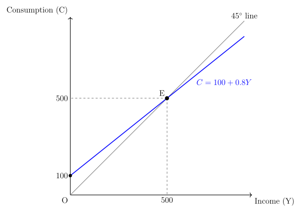
Start your 14-day free trial to see the full solution →
CBSE 2026Set 58/2/11 markMCQ
$Q. Choose the correct consumption function from the options given below with reference to the illustrated given diagram. (Diagram: X-axis = Income, Y-axis = Consumption; a 45° Income Line; a consumption curve C with a positive intercept of 100; equilibrium point E where the C curve cuts the 45° line; dashed lines mark C = 280 at one income level and C = 700 at income = 800.) Options : (A) C = 100 + 0.7Y (B) C = 100 + 0.8Y (C) C = 100 - 0.7Y (D) C = 100 - 0.8Y$
›Reveal solutionSolution

The consumption curve has autonomous consumption $\bar{C}=100$ (its vertical intercept) and its slope is the MPC. Using the break-even point $E$ where the curve cuts the $45°$ line ( $C=Y=500$ ), the MPC works out to exactly $0.8$ , so the consumption function is $C = 100 + 0.8Y$ — option (B).

The consumption function and its components

A consumption function describes the relationship between national income $Y$ and aggregate consumption $C$ . The standard Keynesian form is
$C = \bar{C} + c \, Y$
where $\bar{C}$ is autonomous consumption (consumption when income is zero — the vertical intercept) and $c$ is the marginal propensity to consume (MPC), the fraction of each additional rupee of income spent on consumption, and geometrically the slope of the line.

The diagram gives us two facts. First, the consumption curve has a positive vertical intercept of $100$ , so $\bar{C} = 100$ . Second, the curve is upward-sloping, which immediately rules out options (C) and (D): a negative coefficient would mean consumption falls as income rises, contradicting both theory and the diagram.

Finding the MPC from the break-even point

The cleanest way to read the slope off this diagram is the break-even point $E$ , where the consumption curve intersects the $45°$ line. Along the $45°$ line every point satisfies $C = Y$ , so at $E$ consumption exactly equals income. From the diagram, this occurs at $Y = C = 500$ .

Substituting $\bar{C} = 100$ and the point $(Y, C) = (500, 500)$ into $C = \bar{C} + cY$ :
$500 = 100 + c(500)$ $400 = 500c$
$c = \frac{400}{500} = 0.8$ …
Start your 14-day free trial to see the full solution →
CBSE 2026Set 58/2/11 markMCQ
$Q. The Aggregate Demand (AD) curve lies parallel to consumption curve, indicating that both have ________. (Choose the correct option to fill in the blank) (A) same components (B) different slope (C) same slope (D) inverse relationship$
›Reveal solutionSolution
The Aggregate Demand (AD) curve is derived by vertically shifting the consumption curve upwards by the amount of autonomous expenditures; since these additions are independent of income, the slope of the AD curve remains the same as the slope of the consumption curve, which is the Marginal Propensity to Consume (MPC).

To understand why the Aggregate Demand (AD) curve lies parallel to the consumption curve, we need to examine the components and slopes of both.

First, let's consider the consumption function. In Keynesian economics, the consumption function describes the relationship between consumption expenditure and disposable income. It is typically represented as:

$C = \bar{C} + bY$

where:

$C$ is total consumption expenditure.

$\bar{C}$ is autonomous consumption (consumption that occurs even when income is zero).

$b$ is the Marginal Propensity to Consume (MPC), which is the change in consumption for a unit change in income ( $\Delta C / \Delta Y$ ).

$Y$ is disposable income.

The slope of the consumption curve is given by $b$ , the Marginal Propensity to Consume. This value indicates how much of an additional rupee of income is spent on consumption.

Next, let's look at the Aggregate Demand (AD) function. Aggregate Demand represents the total demand for goods and services in an economy at a given price level. In a simple two-sector economy (households and firms), AD is the sum of consumption (C) and investment (I):

$AD = C + I$

Substituting the consumption function into the AD equation:

$AD = (\bar{C} + bY) + I$

In this simplified model, investment ( $I$ ) is often assumed to be autonomous, meaning it does not depend on the level of income. It is determined by factors like interest rates, business expectations, and government policy. Therefore, $I$ is a constant value.

We can rearrange the AD function as:

$AD = (\bar{C} + I) + bY$
$AD = (\bar{C} + I) + bY$
Start your 14-day free trial to see the full solution →
CBSE 2026Set 58/3/11 markMCQ
$Q. Identify the variable(s) which may add to the future productive capacity of an economy : I. Raw material II. Fixed investment III. Inventories with producers (Choose the correct option) Options : (A) Only I (B) Only II (C) II and III (D) I, II and III$
›Reveal solutionSolution

Future productive capacity grows through additions to the capital stock that enable more output tomorrow. Only fixed investment (II) and inventories with producers (III) qualify; raw materials are intermediate inputs consumed in current production.

The question asks which variables add to future productive capacity—in other words, which items expand the economy's ability to produce goods and services in periods ahead. This is fundamentally about capital accumulation, not current consumption of inputs.

I. Raw material

Raw materials are intermediate goods purchased by firms to be transformed into final products within the same accounting period. When a bakery buys flour, that flour is used up immediately in making bread; it does not sit as a durable asset that raises the bakery's capacity next year. Raw materials flow through production rather than augmenting the stock of productive assets. They are part of the cost of goods sold, not an addition to capital.

Watch out

A common confusion: raw materials are essential for production, but they do not add to capacity—they are consumed in the act of producing. Capacity depends on the stock of machines, buildings, and usable inventories, not on inputs that vanish in the production process.

II. Fixed investment

Fixed investment—expenditure on machinery, equipment, buildings, and infrastructure—directly increases the capital stock. A new lathe in a workshop, a factory extension, or a fleet of trucks all raise the maximum output the economy can sustain. These assets are durable; they contribute to production over many periods. This is the textbook channel through which an economy builds future capacity.

III. Inventories with producers

Inventories held by producers (unsold finished goods, work-in-progress, and raw materials not yet used) are classified as investment in national accounts precisely because they represent output that has been produced but not yet sold or consumed. Crucially, a stock of inventories allows a firm to smooth production and meet future demand without delay. If a car manufacturer holds 500 finished cars in stock, those cars can be sold next quarter without requiring new production runs—effectively, the inventory acts as a buffer that sustains sales (and hence productive activity) even when current production dips. In this sense, inventories are a form of capital that supports future output. …
Start your 14-day free trial to see the full solution →
CBSE 2026Set 58/3/11 markMCQ
$Q. Select the correct formula to calculate the value of Marginal Propensity to Save (MPS) : I. Change in Savings (ΔS) / Change in Consumption (ΔC) II. Change in Savings (ΔS) / Change in Income (ΔY) III. 1 - Marginal Propensity to Consume (MPC) IV. Change in Income (ΔY) / Change in Savings (ΔS) Options : (A) I, II, III and IV (B) II and III (C) Only III (D) Only II$
›Reveal solutionSolution

MPS measures the fraction of additional income that households save rather than consume. The correct formulas are II (ΔS/ΔY, the definition) and III (1 – MPC, from the income identity), so the answer is (B).

The Marginal Propensity to Save captures a simple behavioral question: when your income rises by one rupee, how much of that extra rupee do you tuck away as savings? It's the savings counterpart to the Marginal Propensity to Consume.

Start with the fundamental income identity. Every rupee of additional income must be either consumed or saved—there is no third bucket. Mathematically, for any change in income:
$\Delta Y = \Delta C + \Delta S$
Divide both sides by $\Delta Y$ :
$\frac{\Delta Y}{\Delta Y} = \frac{\Delta C}{\Delta Y} + \frac{\Delta S}{\Delta Y}$ $1 = \text{MPC} + \text{MPS}$
This tells us immediately that MPS = 1 – MPC (option III is correct). If households consume 0.75 of each additional rupee, they must save the remaining 0.25; the two propensities are complementary fractions of the same whole.
$\text{MPS} = \frac{\Delta S}{\Delta Y} = 1 - \text{MPC}$
Now examine the definition. MPS is the responsiveness of savings to income, so by definition it is the ratio of the change in savings to the change in income that caused it: ΔS/ΔY (option II is correct). This is the direct, textbook definition—just as MPC is ΔC/ΔY, MPS is ΔS/ΔY. …
Start your 14-day free trial to see the full solution →
CBSE 2026Set 58/3/11 markMCQ
$Q. Read the following statements carefully : Statement I : At the break-even level of income, the value of slope of the consumption curve is zero. Statement II : Marginal Propensity to Consume (MPC) refers to the change in consumption per unit change in income. In the light of the given statements, choose the correct option from the following : (A) Statement I is true and Statement II is false. (B) Statement I is false and Statement II is true. (C) Both Statements I and II are true. (D) Both Statements I and II are false.$
›Reveal solutionSolution

Statement I is false because the slope of the consumption curve at break-even income is the MPC, which is positive (not zero). Statement II is true because MPC is defined as the change in consumption per unit change in income.

Let’s unpack this carefully. The question tests two distinct ideas from the theory of consumption and income determination — the break-even point and the meaning of Marginal Propensity to Consume (MPC).

Statement I talks about the break-even level of income. In macroeconomics, the break-even point is that level of income where consumption exactly equals income — so saving is zero. At this point, the consumption curve (which plots consumption against income) is not flat; it has a positive slope. Why? Because the consumption function is typically written as $C = \bar{C} + bY$ , where $\bar{C}$ is autonomous consumption (positive even at zero income) and $b$ is the MPC — the slope of the curve. At break-even, $C = Y$ , so $\bar{C} + bY = Y$ , which gives $Y = \bar{C} / (1-b)$ . The slope here is still $b$ , which is a positive fraction (between 0 and 1). It is never zero unless MPC is zero, which would mean consumption never changes with income — a situation that contradicts the basic Keynesian consumption function. So Statement I is false.

Note

A common confusion: students sometimes think “break-even” means the curve is horizontal. But break-even is about the level of income where C = Y, not about the slope. The slope remains the MPC throughout. …

Start your 14-day free trial to see the full solution →
CBSE 2026Set MARCH1 markMCQ
$Q. Rate of change in savings as income increases is$
(a) Average propensity to consume
(b) Average propensity to save
(c) Marginal propensity to save
(d) Marginal propensity to consume
›Reveal solutionSolution

The rate of change in saving as income changes is the marginal propensity to save, so the answer is (c).

…

Start your 14-day free trial to see the full solution →
CBSE 2026Set MARCH1 mark
$Q.__________ is defined as addition to the stock of physical capital.$
›Reveal solutionSolution

The blank is filled by Investment.

Investment (capital formation) is the addition made during a year to the existing stock of physical capital such as machinery, buildings, tools and inventories. It is a flow that increases the economy's productive capacity. When we add new capital goods and the change in inventories to the …

Start your 14-day free trial to see the full solution →
CBSE 2026Set ANNUAL1 markMCQ
$Q. The consumer does not change his consumption despite change in his income, than the value of MPC will be A) MPC > 1 B) MPC = 1 C) MPC = 0 D) MPC < 1$
›Reveal solutionSolution

No change in consumption when income changes means MPC = 0, so the answer is C.

Marginal Propensity to Consume (MPC) = change in consumption (ΔC) ÷ change in income (ΔY). The question states the consumer does not change consumption despite a change in income, so ΔC = 0. Therefore MPC = 0 ÷ ΔY = 0. Values like MPC > …

Start your 14-day free trial to see the full solution →
CBSE 2026Set ANNUAL1 markMCQ
$Q. Formula of consumption function is A) C = C̄ - cY B) C = C̄ + cY C) C = S̄ - cY D) C = S̄ + cY$
›Reveal solutionSolution

The consumption function is C = C̄ + cY, so the answer is B.

In the Keynesian consumption function, C̄ is autonomous consumption (the consumption that takes place even at zero income) and c is the marginal propensity to consume, so cY is the induced consumption that rises with income Y. Consumption therefore increases with incom …

Start your 14-day free trial to see the full solution →
CBSE 2026Set ANNUAL1 mark
$Q. Define the average propensity to consume.$
›Reveal solutionSolution

APC is total consumption divided by total income: APC = C/Y.

The Average Propensity to Consume (APC) measures the proportion of total income that households spend on consumption. It is defined as APC = C ÷ Y, where C is total consumption expenditure and Y is total (disposable) income. For example, if income is ₹1,000 and consumption is ₹800, then APC = 800 ÷ 1,000 = 0.8, meaning 80% of income is consumed. This is a standard definition in the Class-12 …

Start your 14-day free trial to see the full solution →
CBSE 2026Set ANNUAL1 mark
$Q. Find the value of MPS, if the MPC = 0.75.$
›Reveal solutionSolution

MPS = 1 − MPC = 1 − 0.75 = 0.25.

Any additional unit of income is either consumed or saved, so the marginal propensity to consume (MPC) and the marginal propensity to save (MPS) always add up to 1: MPC + MPS = 1. Given MPC = 0.75:

| Step | Working |

|---|---| …

Start your 14-day free trial to see the full solution →

←Previous questionQ63 — For a hypothetical economy, assume the government increased an infrast…→Next questionQ65 — Read the following statements : Assertion (A) and Reason (R). Choose t…

Part (a)

🎓Unlock everything free for 14 days

Unlock everything free for 14 days