Maxima and Minima

Definition 3Maximum / minimum value of a function on an interval

Maximum and minimum value of a function on an interval

Let $f$ be a function defined on an interval $I$ .

(a) Maximum value. $f$ has a maximum value on $I$ if there is a point $c \in I$ such that

f(c) \ge f(x) \quad \text{for all } x \in I.

The number $f(c)$ is the maximum value of $f$ on $I$ , and $c$ is a point of maximum value.

(b) Minimum value. $f$ has a minimum value on $I$ if there is a point $d \in I$ such that

f(d) \le f(x) \quad \text{for all } x \in I.

The number $f(d)$ is the minimum value of $f$ on $I$ , and $d$ is a point of minimum value.

(c) Extreme value. $f$ is said to have an extreme value on $I$ if it has either a maximum value or a minimum value on $I$ ; the point where this happens is an extreme point.

Key idea: Here the comparison is over the entire interval $I$ — the largest (or smallest) output beats every other output, not just nearby ones.

Tiny Concrete Example …

Definition 4Point of local maxima / local minima

Definition of Local Maxima and Local Minima

Let $f$ be a real-valued function, and let $c$ be an interior point in the domain of $f$ (meaning there is an open interval around $c$ that lies entirely inside the domain).

(a) Point of Local Maxima $c$ is called a point of local maxima if there exists some $h > 0$ such that

f(c) \ge f(x) \quad \text{for all } x \text{ in } (c - h, c + h), \; x \neq c.

The value $f(c)$ is called the local maximum value of $f$ .

(b) Point of Local Minima $c$ is called a point of local minima if there exists some $h > 0$ such that

f(c) \le f(x) \quad \text{for all } x \text{ in } (c - h, c + h), \; x \neq c.

The value $f(c)$ is called the local minimum value of $f$ .

(c) Extreme Value $f$ is said to have an extreme value at $c$ if $f(c)$ is either a local maximum or a local minimum value.

Intuition

A point of local maxima is the top of a little hill — the function is higher at $c$ than at any nearby point. A point of local minima is the bottom of a little valley — the function is lower at $c$ than at any nearby point. The $h$ simply defines a small neighbourhood around $c$ where this comparison holds. …

Theorem 2

The Second Derivative Test

When you have a function $f$ and you want to find its local maxima and minima, the first derivative test works by checking how $f'$ changes sign around a critical point. The second derivative test gives you a faster way — it looks at the curvature of the graph at that point.

Statement of the Theorem

f

The hypotheses are precise: $f$ must be defined on an interval containing $c$ , and the second derivative must exist at $c$ itself. The condition $f'(c) = 0$ tells you $c$ is a critical point; the sign of $f''(c)$ then tells you whether the graph is curving downward (local max) or upward (local min) at that point.

Watch out

The second derivative test only works when $f''(c) \neq 0$ . If $f''(c) = 0$ , the test gives no information — the point could be a local max, local min, or a point of inflection. You must then use the first derivative test.

Complete Proof

›Proof

We prove part (i): $f'(c) = 0$ and $f''(c) < 0$ implies $x = c$ is a point of local maxima. Part (ii) is proved similarly.

Step 1: Write the definition of the second derivative.

Since $f$ is twice differentiable at $c$ , the second derivative exists and is given by the limit:

$f''(c) = \lim_{x \to c} \frac{f'(x) - f'(c)}{x - c}$

Step 2: Use the given condition $f'(c) = 0$ .

Substituting $f'(c) = 0$ , we get:

$f''(c) = \lim_{x \to c} \frac{f'(x)}{x - c}$

Step 3: Apply the hypothesis $f''(c) < 0$ .

Since $f''(c) < 0$ , the limit above is negative. By the definition of a limit, there exists some $h > 0$ such that for all $x$ in the deleted neighbourhood $(c - h, c + h)$ , $x \neq c$ , we have:

$\frac{f'(x)}{x - c} < 0$

This is the key inequality that will determine the sign of $f'(x)$ on either side of $c$ .

Step 4: Analyse the sign of $f'(x)$ to the left of $c$ .

Take any $x$ such that $c - h < x < c$ . Then $x - c < 0$ . For the fraction $\frac{f'(x)}{x - c}$ to be negative (as required), the numerator $f'(x)$ must be positive (since a positive divided by a negative gives a negative). Therefore:

$f'(x) > 0 \quad \text{for all } x \in (c - h, c)$

This means $f$ is increasing immediately to the left of $c$ .

Step 5: Analyse the sign of $f'(x)$ to the right of $c$ .

Now take any $x$ such that $c < x < c + h$ . Then $x - c > 0$ . For the fraction $\frac{f'(x)}{x - c}$ to be negative, the numerator $f'(x)$ must be negative (since a negative divided by a positive gives a negative). Therefore:

$f'(x) < 0 \quad \text{for all } x \in (c, c + h)$

This means $f$ is decreasing immediately to the right of $c$ .

Step 6: Apply the first derivative test.

We have shown that $f'(x)$ changes sign from positive (to the left of $c$ ) to negative (to the right of $c$ ) as $x$ increases through $c$ . By the First Derivative Test (Theorem 3), this is exactly the condition for $x = c$ to be a point of local maxima. Hence $f(c)$ is a local maximum value of $f$ .

Proof of part (ii): If $f''(c) > 0$ , the same reasoning gives $\frac{f'(x)}{x - c} > 0$ near $c$ . Then:

For $x < c$ : $x - c < 0$ , so $f'(x) < 0$ (function decreasing to the left)
For $x > c$ : $x - c > 0$ , so $f'(x) > 0$ (function increasing to the right)

This sign change (negative to positive) is precisely the first derivative test condition for a local minimum.

…

Theorem 3

The Second Derivative Test

When you have a function $f$ and you want to find its local maxima and minima, the first derivative test works by checking how $f'$ changes sign around a critical point. The second derivative test gives you a faster way — it looks at the curvature of the graph at that point.

Statement of the Theorem

f

The hypotheses are precise: $f$ must be defined on an interval containing $c$ , and the second derivative must exist at $c$ itself. The condition $f'(c) = 0$ tells you $c$ is a critical point; the sign of $f''(c)$ then tells you whether the graph is curving downward (local max) or upward (local min) at that point.

Watch out

The second derivative test only works when $f''(c) \neq 0$ . If $f''(c) = 0$ , the test gives no information — the point could be a local max, local min, or a point of inflection. You must then use the first derivative test.

Complete Proof

›Proof

We prove part (i): $f'(c) = 0$ and $f''(c) < 0$ implies $x = c$ is a point of local maxima. Part (ii) is proved similarly.

Step 1: Write the definition of the second derivative.

Since $f$ is twice differentiable at $c$ , the second derivative exists and is given by the limit:

$f''(c) = \lim_{x \to c} \frac{f'(x) - f'(c)}{x - c}$

Step 2: Use the given condition $f'(c) = 0$ .

Substituting $f'(c) = 0$ , we get:

$f''(c) = \lim_{x \to c} \frac{f'(x)}{x - c}$

Step 3: Apply the hypothesis $f''(c) < 0$ .

Since $f''(c) < 0$ , the limit above is negative. By the definition of a limit, there exists some $h > 0$ such that for all $x$ in the deleted neighbourhood $(c - h, c + h)$ , $x \neq c$ , we have:

$\frac{f'(x)}{x - c} < 0$

This is the key inequality that will determine the sign of $f'(x)$ on either side of $c$ .

Step 4: Analyse the sign of $f'(x)$ to the left of $c$ .

Take any $x$ such that $c - h < x < c$ . Then $x - c < 0$ . For the fraction $\frac{f'(x)}{x - c}$ to be negative (as required), the numerator $f'(x)$ must be positive (since a positive divided by a negative gives a negative). Therefore:

$f'(x) > 0 \quad \text{for all } x \in (c - h, c)$

This means $f$ is increasing immediately to the left of $c$ .

Step 5: Analyse the sign of $f'(x)$ to the right of $c$ .

Now take any $x$ such that $c < x < c + h$ . Then $x - c > 0$ . For the fraction $\frac{f'(x)}{x - c}$ to be negative, the numerator $f'(x)$ must be negative (since a negative divided by a positive gives a negative). Therefore:

$f'(x) < 0 \quad \text{for all } x \in (c, c + h)$

This means $f$ is decreasing immediately to the right of $c$ .

Step 6: Apply the first derivative test.

We have shown that $f'(x)$ changes sign from positive (to the left of $c$ ) to negative (to the right of $c$ ) as $x$ increases through $c$ . By the First Derivative Test (Theorem 3), this is exactly the condition for $x = c$ to be a point of local maxima. Hence $f(c)$ is a local maximum value of $f$ .

Proof of part (ii): If $f''(c) > 0$ , the same reasoning gives $\frac{f'(x)}{x - c} > 0$ near $c$ . Then:

For $x < c$ : $x - c < 0$ , so $f'(x) < 0$ (function decreasing to the left)
For $x > c$ : $x - c > 0$ , so $f'(x) > 0$ (function increasing to the right)

This sign change (negative to positive) is precisely the first derivative test condition for a local minimum.

…

Theorem 4

The Second Derivative Test

When you have a function $f$ and you want to find its local maxima and minima, the first derivative test works by checking how $f'$ changes sign around a critical point. The second derivative test gives you a faster way — it looks at the curvature of the graph at that point.

Statement of the Theorem

f

The hypotheses are precise: $f$ must be defined on an interval containing $c$ , and the second derivative must exist at $c$ itself. The condition $f'(c) = 0$ tells you $c$ is a critical point; the sign of $f''(c)$ then tells you whether the graph is curving downward (local max) or upward (local min) at that point.

Watch out

The second derivative test only works when $f''(c) \neq 0$ . If $f''(c) = 0$ , the test gives no information — the point could be a local max, local min, or a point of inflection. You must then use the first derivative test.

Complete Proof

›Proof

We prove part (i): $f'(c) = 0$ and $f''(c) < 0$ implies $x = c$ is a point of local maxima. Part (ii) is proved similarly.

Step 1: Write the definition of the second derivative.

Since $f$ is twice differentiable at $c$ , the second derivative exists and is given by the limit:

$f''(c) = \lim_{x \to c} \frac{f'(x) - f'(c)}{x - c}$

Step 2: Use the given condition $f'(c) = 0$ .

Substituting $f'(c) = 0$ , we get:

$f''(c) = \lim_{x \to c} \frac{f'(x)}{x - c}$

Step 3: Apply the hypothesis $f''(c) < 0$ .

Since $f''(c) < 0$ , the limit above is negative. By the definition of a limit, there exists some $h > 0$ such that for all $x$ in the deleted neighbourhood $(c - h, c + h)$ , $x \neq c$ , we have:

$\frac{f'(x)}{x - c} < 0$

This is the key inequality that will determine the sign of $f'(x)$ on either side of $c$ .

Step 4: Analyse the sign of $f'(x)$ to the left of $c$ .

Take any $x$ such that $c - h < x < c$ . Then $x - c < 0$ . For the fraction $\frac{f'(x)}{x - c}$ to be negative (as required), the numerator $f'(x)$ must be positive (since a positive divided by a negative gives a negative). Therefore:

$f'(x) > 0 \quad \text{for all } x \in (c - h, c)$

This means $f$ is increasing immediately to the left of $c$ .

Step 5: Analyse the sign of $f'(x)$ to the right of $c$ .

Now take any $x$ such that $c < x < c + h$ . Then $x - c > 0$ . For the fraction $\frac{f'(x)}{x - c}$ to be negative, the numerator $f'(x)$ must be negative (since a negative divided by a positive gives a negative). Therefore:

$f'(x) < 0 \quad \text{for all } x \in (c, c + h)$

This means $f$ is decreasing immediately to the right of $c$ .

Step 6: Apply the first derivative test.

We have shown that $f'(x)$ changes sign from positive (to the left of $c$ ) to negative (to the right of $c$ ) as $x$ increases through $c$ . By the First Derivative Test (Theorem 3), this is exactly the condition for $x = c$ to be a point of local maxima. Hence $f(c)$ is a local maximum value of $f$ .

Proof of part (ii): If $f''(c) > 0$ , the same reasoning gives $\frac{f'(x)}{x - c} > 0$ near $c$ . Then:

For $x < c$ : $x - c < 0$ , so $f'(x) < 0$ (function decreasing to the left)
For $x > c$ : $x - c > 0$ , so $f'(x) > 0$ (function increasing to the right)

This sign change (negative to positive) is precisely the first derivative test condition for a local minimum.

…

Figure 6.7Three graphs (a), (b), (c) showing the value f(c) at a local maximum, a point of non-differentiability, and a local minimum

Fig. 6.7 — Three graphs (a), (b), (c) showing the value f(c) at a local maximum, a point of non-differentiability, and a local minimum

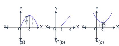
Drawn by us to help you understand the concept clearly, and verified to make sure it's accurate. For exams, practice from your NCERT textbook's own diagram.

What Fig. 6.7 Teaches: The Three Faces of Extreme Values

The figure is a triptych — three separate Cartesian panels, each with labelled axes $X'\!-\!O\!-\!X$ and $Y'\!-\!O\!-\!Y$ — designed to show the three fundamentally different ways a function can achieve a maximum or minimum value. The core idea is that extreme values can occur at a peak or trough inside an interval, at an endpoint of the interval, or at a point where the function is not differentiable. Each panel illustrates one of these cases.

Panel (a): The Interior Peak (Local Maximum)

A smooth, downward-opening indigo arch rises to a single highest point, then falls. A solid vertical line drops from that peak straight down to the $x$ -axis, landing at a point labelled $c$ . Dashed vertical guide lines flank this solid line, emphasising that $c$ lies strictly between the ends of the interval shown. The height of the peak is labelled $f(c)$ .

This panel teaches the classical local maximum: the function is differentiable at $c$ , the derivative $f'(c)=0$ , and the graph changes from increasing to decreasing as we pass through $c$ . The value $f(c)$ is larger than every other value in some neighbourhood around $c$ .

Panel (b): The Endpoint Maximum

A rising straight indigo segment runs from $x=1$ to $x=4$ on the $x$ -axis. A dashed vertical line drops from the right endpoint at $x=4$ down to the axis. The maximum occurs at the endpoint of the interval, not at an interior turning point.

This panel illustrates that when a function is monotonic (here, strictly increasing) on a closed interval, the maximum is found at the right endpoint and the minimum at the left endpoint. No derivative test is needed — the extreme values are simply the function values at the boundaries.

Panel (c): The Interior Minimum (Local Minimum)

An upward-opening indigo parabola sits above the $x$ -axis, with its vertex — the lowest point — directly above a point $c$ on the $x$ -axis. Dashed guide lines again frame $c$ , and the minimum height is labelled $f(c)$ .

This is the mirror image of panel (a): a local minimum where $f'(c)=0$ , the derivative changes from negative to positive, and $f(c)$ is smaller than all nearby values.

Note

The textbook's Remark explicitly states that these graphs help us find maximum/minimum values even at points where the function is not differentiable (Example 15, $f(x)=|x|$ , is cited). Panel (c) could also represent such a case — the parabola is smooth, but the concept of a minimum at a cusp or corner is visually analogous.

The Key Formula the Figure Supports

The figure directly motivates the First Derivative Test (Theorem 3). For a critical point $c$ (where $f'(c)=0$ or $f$ is not differentiable):

\begin{aligned} &\text{Local maximum at }c \quad\text{if } f'(x) > 0 \text{ for } x < c \text{ and } f'(x) < 0 \text{ for } x > c.\\[4pt] &\text{Local minimum at }c \quad\text{if } f'(x) < 0 \text{ for } x < c \text{ and } f'(x) > 0 \text{ for } x > c. \end{aligned}

Here:

$f'(x)$ is the derivative (rate of change) of the function.
$c$ is the point on the $x$ -axis where the extreme value occurs.
$f(c)$ is the extreme value itself — the height of the peak or depth of the trough. …

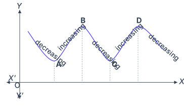
Figure 6.11Graph whose nature changes (turning points A, B, C, D)

Fig. 6.11 — Graph whose nature changes (turning points A, B, C, D)

Drawn by us to help you understand the concept clearly, and verified to make sure it's accurate. For exams, practice from your NCERT textbook's own diagram.

What Fig. 6.11 Shows

The figure presents a single smooth, indigo-coloured curve drawn above the X-axis on a standard Cartesian plane with axes X′–O–X and Y′–O–Y. The curve is wavy: it begins by falling, reaches a valley at point A, rises to a hill at B, falls again to a valley at C, rises to a hill at D, and finally descends once more. The four turning points — A, B, C, D — are clearly labelled on the curve. Dashed vertical lines drop from each turning point down to the X-axis, helping you read the x-coordinate of each extremum.

The five monotonic (purely increasing or purely decreasing) stretches between these points carry slanted labels — 'decreasing' or 'increasing' — that follow the slope of the curve. This visual cue makes it immediate which way the function is moving on each interval.

The Physical Idea

The core concept is that a function's behaviour changes at certain special points. Before a local maximum, the function rises (increasing); after it, the function falls (decreasing). Before a local minimum, the function falls; after it, the function rises. These points where the monotonic nature flips are called turning points. In Fig. 6.11, A and C are local minima (the bottoms of valleys), while B and D are local maxima (the tops of hills). The curve does not have to be differentiable at a turning point — but in this smooth example, it is.

The textbook uses this figure to introduce the idea that at a turning point, the derivative is zero (provided the function is differentiable there). This is the geometric foundation for the First Derivative Test and the Second Derivative Test.

The Key Result Developed from This Figure

The central theorem that Fig. 6.11 motivates is:

f

In Fig. 6.11, at point B (a local maximum), the curve is increasing just before B and decreasing just after B — so $f'(x)$ goes from positive to negative. At point A (a local minimum), the curve is decreasing just before A and increasing just after A — so $f'(x)$ goes from negative to positive.

The textbook also introduces the Second Derivative Test as an alternative: if $f'(c)=0$ and $f''(c)<0$ , then $c$ is a local maximum; if $f'(c)=0$ and $f''(c)>0$ , then $c$ is a local minimum. If $f''(c)=0$ , the test fails and you must use the first derivative test.

Watch out

A zero derivative does not guarantee a turning point. For example, $f(x)=x^3$ has $f'(0)=0$ but 0 is a point of inflection, not a local extremum. Always check the sign change of $f'(x)$ or the value of $f''(x)$ .

How the Figure Connects to the Definitions …

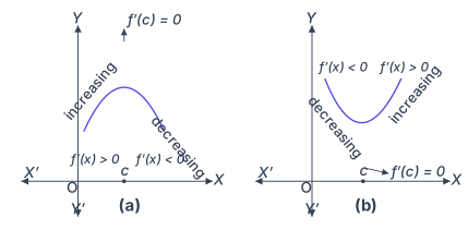
Figure 6.12Graph of f around a point of local maxima (a) and local minima (b)

Fig. 6.12 — Graph of f around a point of local maxima (a) and local minima (b)

Drawn by us to help you understand the concept clearly, and verified to make sure it's accurate. For exams, practice from your NCERT textbook's own diagram.

What Fig. 6.12 Shows

The figure presents two separate Cartesian plots side by side, labelled (a) and (b). Each plot has the standard axes: the horizontal axis is labelled X′–O–X (the $x$ -axis) and the vertical axis Y′–O–Y (the $y$ -axis), with the origin at O. The point $c$ is marked on the $x$ -axis in both panels, directly below a special point on the curve.

Panel (a) shows a smooth, hill-shaped curve (an inverted U, or $\cap$ -shape). The left side of the hill rises as we move toward $c$ ; this branch is labelled increasing and carries the condition $f'(x) > 0$ . The right side falls away from $c$ ; it is labelled decreasing and carries $f'(x) < 0$ . At the very top of the hill — directly above $c$ — an upward-pointing arrow reads $f'(c) = 0$ . This panel illustrates a point of local maximum.

Panel (b) shows a smooth, valley-shaped curve (a U-shape, or $\cup$ -shape). The left side falls as we approach $c$ ; it is labelled decreasing with $f'(x) < 0$ . The right side rises away from $c$ ; it is labelled increasing with $f'(x) > 0$ . At the bottom of the valley — directly above $c$ — an arrow reads $f'(c) = 0$ . This panel illustrates a point of local minimum.

The two panels together make a single conceptual point: at a turning point where the graph changes from rising to falling (or falling to rising), the derivative must be zero, provided the function is differentiable there.

The Physical Idea

A function that is smooth (differentiable) cannot have a peak or a trough without first "flattening out" at the very top or bottom. Imagine walking up a hill: your slope (the derivative) is positive as you climb. At the summit, for an instant, the ground is level — your slope is zero. As you descend the other side, the slope becomes negative. The same logic applies in reverse for a valley: you descend (negative slope), reach a flat point (zero slope), then ascend (positive slope).

The figure makes this geometric intuition precise. The derivative $f'(x)$ tells us the slope of the tangent line at any point. Where the slope changes sign — from positive to negative, or negative to positive — the function must pass through a point where the slope is exactly zero. That point is a candidate for a local extremum.

Watch out

A zero derivative does not guarantee a local maximum or minimum. The function $f(x) = x^3$ has $f'(0) = 0$ , but the graph has no peak or valley at $x = 0$ — it simply flattens momentarily and continues rising. Such a point is called a point of inflection. The sign change of $f'(x)$ around $c$ is what confirms whether $c$ is truly a local extremum.

The Key Formula and Its Meaning

The central result that Fig. 6.12 introduces is the First Derivative Test for local maxima and minima. Let $f$ be continuous at a critical point $c$ (where $f'(c) = 0$ or $f$ is not differentiable). Then:

\begin{aligned} &\text{Local maximum at }c \quad\text{if}\quad f'(x) > 0 \text{ for } x < c \text{ (near }c\text{)} \;\text{and}\; f'(x) < 0 \text{ for } x > c \text{ (near }c\text{)}. \\[4pt] &\text{Local minimum at }c \quad\text{if}\quad f'(x) < 0 \text{ for } x < c \text{ (near }c\text{)} \;\text{and}\; f'(x) > 0 \text{ for } x > c \text{ (near }c\text{)}. \end{aligned}

In the figure, panel (a) shows the first case: $f'(x)$ goes from positive (left of $c$ ) to zero (at $c$ ) to negative (right of $c$ ). Panel (b) shows the second case: $f'(x)$ goes from negative to zero to positive.

The symbols have these meanings:

$f(x)$ — the function whose graph is drawn.
$f'(x)$ — the first derivative of $f$ , giving the slope of the tangent at any point $x$ .
$c$ — a point in the domain of $f$ where the derivative is zero (a critical point). …

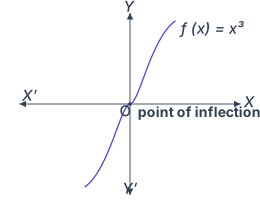
Figure 6.13Graph of f(x) = x³ with point of inflection at O

Fig. 6.13 — Graph of f(x) = x³ with point of inflection at O

Drawn by us to help you understand the concept clearly, and verified to make sure it's accurate. For exams, practice from your NCERT textbook's own diagram.

What Fig. 6.13 Shows

The graph is a simple Cartesian plot with axes labelled X′–O–X (horizontal) and Y′–O–Y (vertical), both with arrowheads. The origin is marked O. A single smooth indigo curve rises from the lower-left quadrant (third quadrant), passes through the origin, and continues into the upper-right quadrant (first quadrant). The curve is labelled f(x) = x³ near its upper-right branch.

At the origin, the curve has a flat horizontal tangent — the tangent line is drawn (or implied) to be horizontal at O. The point O itself is labelled "point of inflection". For $x < 0$ , the curve is concave down (curving downward like an upside-down bowl). For $x > 0$ , it is concave up (curving upward like a right-side-up bowl).

The Physical Idea

This figure teaches a critical nuance in the study of maxima and minima. The derivative at the origin is zero:

f'(x) = 3x^2 \quad \Rightarrow \quad f'(0) = 0

Yet the origin is neither a local maximum nor a local minimum. The function does not have a "hill" or a "valley" at $x = 0$ — it simply flattens momentarily and continues rising. This is the classic counterexample to the naive belief that a zero derivative always signals a turning point.

The figure illustrates Theorem 3 (First Derivative Test) from the textbook: if $f'(x)$ does not change sign as $x$ increases through a critical point, then that point is neither a local maximum nor a local minimum — it is a point of inflection.

Key Formula and Its Meaning

The central formula the textbook develops with this figure is:

f(x) = x^3

where:

$f(x)$ is the function value (vertical coordinate)
$x$ is the independent variable (horizontal coordinate)

The derivative is:

f'(x) = 3x^2

The second derivative is:

f''(x) = 6x

At $x = 0$ :

$f'(0) = 0$ — the tangent is horizontal
$f''(0) = 0$ — the second derivative test fails (Theorem 4, part (iii)) …

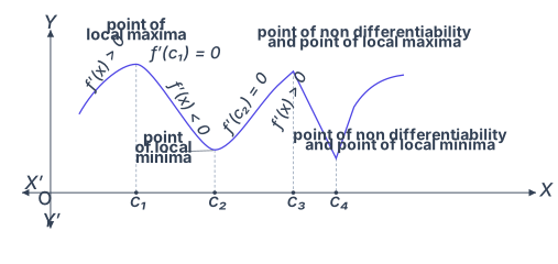
Figure 6.14Critical points c₁, c₂, c₃, c₄ (smooth maxima/minima and non-differentiable cusps)

Fig. 6.14 — Critical points c₁, c₂, c₃, c₄ (smooth maxima/minima and non-differentiable cusps)

Drawn by us to help you understand the concept clearly, and verified to make sure it's accurate. For exams, practice from your NCERT textbook's own diagram.

Understanding Fig. 6.14: Critical Points and the First Derivative Test

This figure is the visual anchor for one of the most important ideas in the chapter: a critical point is not always a smooth turning point. The graph shows a single continuous curve on the standard Cartesian plane (axes X′–O–X and Y′–O–Y, origin O) that passes through four distinct critical points, each projected down to the x‑axis at labels $c_1$ , $c_2$ , $c_3$ , $c_4$ by dashed vertical guide lines.

What the curve teaches

The curve is deliberately drawn to contrast two kinds of critical points. At $c_1$ and $c_2$ , the function is differentiable and the derivative vanishes — these are the familiar smooth maxima and minima you find by setting $f'(x)=0$ . At $c_3$ and $c_4$ , the function is not differentiable (the graph forms a sharp cusp), yet these points are still local extrema. The figure makes the abstract definition of a critical point — "either $f'(c)=0$ or $f$ is not differentiable at $c$ " — visually concrete.

The four critical points in detail

Over $c_1$ (smooth local maximum): The curve rises to a rounded hilltop, then falls. The derivative sign is written along the curve: $f'(x) > 0$ on the left side (the function is increasing as it approaches $c_1$ ), and $f'(x) < 0$ on the right side (decreasing after $c_1$ ). At the peak itself, $f'(c_1)=0$ .

Over $c_2$ (smooth local minimum): The curve descends into a rounded valley, then rises. The sign pattern is reversed: $f'(x) < 0$ on the approach, $f'(x) > 0$ as it leaves. At the bottom, $f'(c_2)=0$ .

Over $c_3$ (non‑differentiable local maximum): The curve comes up to a sharp point — an upward‑pointing cusp — and then drops steeply. The derivative does not exist at $c_3$ (the left‑hand and right‑hand slopes are different), but the point is still a local maximum because the function values on either side are lower.

Over $c_4$ (non‑differentiable local minimum): A downward‑pointing cusp. The curve falls to this sharp point and then rises again. Again, $f$ is not differentiable at $c_4$ , yet it is a local minimum.

Note

The figure labels $c_3$ and $c_4$ explicitly as "point of non differentiability and point of local maxima/minima". This is the textbook's way of emphasising that differentiability is not required for a point to be a local extremum — only continuity and the definition of "higher than all nearby points" (or lower) matter.

The key formula this figure supports

The figure is the geometric justification for Theorem 2 (First Derivative Test). The test states:

\text{If } f'(x) \text{ changes sign from } + \text{ to } - \text{ at } c, \text{ then } c \text{ is a local maximum.}

The figure shows exactly this sign change for the smooth points $c_1$ and $c_2$ . For the cusps $c_3$ and $c_4$ , the test still works — you examine the sign of $f'(x)$ on either side, even though $f'(c)$ itself does not exist. The sign pattern around $c_3$ is $+$ on the left, $-$ on the right (local max), and around $c_4$ it is $-$ on the left, $+$ on the right (local min).