Applied Mathematics · Ch 6 — Probability Distribution
Normal Distribution
Normal Distribution
All the distributions discussed so far describe a discrete random variable, where every possible value can be listed and assigned its own probability. A continuous random variable — such as height or weight — can take infinitely many values within a range, so it no longer makes sense to assign a probability to each individual value; instead, it is described by a probability density function (PDF).
A continuous random variable is said to follow a normal distribution (or Gaussian distribution) with parameters mean and variance , written , if its probability density function is:
where is the mean and is the standard deviation. The graph of is the familiar bell-shaped probability curve, with a single peak and tails that extend indefinitely on both sides without ever touching the axis.
A normal distribution has several distinctive features worth remembering:
- The mean, median and mode all coincide at the same value.
- The curve has exactly one peak, making the distribution unimodal.
- The curve is symmetric about — exactly half the values lie below the mean and half lie above it.
- The total area under the curve is always equal to , as required of any probability density function.
- The entire shape of the distribution is fully described by just two parameters — the mean and the standard deviation . …
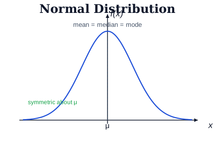
Drawn by us to help you understand the concept clearly, and verified to make sure it's accurate. For exams, practice from your NCERT textbook's own diagram.
The normal curve is a symmetric bell shape; its mean, median and mode all coincide a …