AC Generator

What the Figure Shows

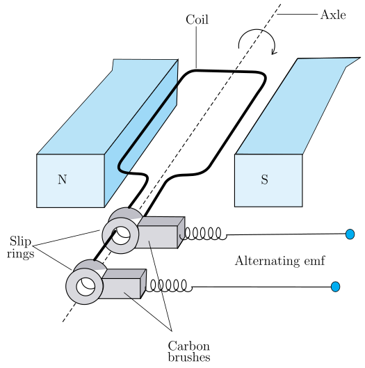
The figure is a schematic 3‑D drawing of a simple AC generator. Its key parts are:

• A rectangular coil (the armature, labelled “Coil”) mounted on a horizontal axle (labelled “Axle”). A dashed line along the axle marks the axis of rotation, and a small curved arrow shows the direction of rotation.
• Two permanent magnet poles: N (left block) and S (right block). The magnetic field $\mathbf{B}$ is uniform and points horizontally from left to right (N → S).
• The two ends of the coil are connected to two slip rings (labelled “Slip rings”) on the shaft. Each slip ring is in contact with a carbon brush (labelled “Carbon brushes”).
• The brushes lead to an external circuit whose terminals are labelled “Alternating emf”.

The coil rotates with constant angular speed $\omega$ inside the uniform field. Because the coil’s orientation changes, the magnetic flux through it varies sinusoidally with time.

---

Physical Idea Taught

The figure illustrates the principle of electromagnetic induction used to generate alternating current. As the coil rotates, the effective area of the coil exposed to the magnetic field changes. The magnetic flux at any instant $t$ is

where:

• $B$ = magnitude of the uniform magnetic field,
• $A$ = area of the coil,
• $\theta = \omega t$ = angle between the area vector $\mathbf{A}$ (normal to the coil) and $\mathbf{B}$ at time $t$ (taking $\theta=0$ when the coil is perpendicular to the field).

By Faraday’s law, the induced emf in a coil of $N$ turns is

The maximum emf (peak value) is

so the instantaneous emf can be written as

Because $\sin\omega t$ alternates between $+1$ and $-1$, the polarity of the emf reverses periodically — this is the alternating emf labelled in the figure. The slip rings and brushes ensure that the external circuit always receives this alternating voltage, regardless of the coil’s rotation.

---

Key Formula Developed with This Figure

The textbook derives the instantaneous induced emf for a rotating coil:

where:

• $N$ = number of turns in the coil,
• $B$ = magnetic field strength (in tesla),
• $A$ = area of the coil (in m²), …

What the Figure Shows

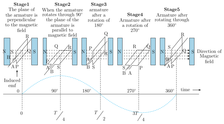
The figure is a composite illustration that connects the physical rotation of a coil in a magnetic field to the alternating emf it generates. The top row shows five schematic stages (Stage 1 through Stage 5) of a rectangular coil (armature) rotating between the north (N) and south (S) poles of a magnet. The coil is labeled with corners P, Q, R, S, and the uniform magnetic field $\mathbf{B}$ points from left (N) to right (S). The stages correspond to successive angular positions of the coil:

• Stage 1 (0°): The plane of the coil is perpendicular to $\mathbf{B}$. The area vector $\mathbf{A}$ (normal to the coil plane) is parallel to $\mathbf{B}$, so the effective area exposed to the field is maximum.
• Stage 2 (90°): The coil plane is parallel to $\mathbf{B}$. $\mathbf{A}$ is perpendicular to $\mathbf{B}$, so the effective area is zero.
• Stage 3 (180°): The coil plane is again perpendicular to $\mathbf{B}$, but now $\mathbf{A}$ is anti-parallel to $\mathbf{B}$ (opposite direction to Stage 1).
• Stage 4 (270°): The coil plane is parallel to $\mathbf{B}$ again, with $\mathbf{A}$ perpendicular to $\mathbf{B}$ (opposite orientation to Stage 2).
• Stage 5 (360°): The coil returns to the same orientation as Stage 1, completing one full rotation.

A note at the far right indicates the direction of the magnetic field.

The bottom part of the figure is a graph with a horizontal axis labeled time (marked with angles $0^\circ$, $90^\circ$, $180^\circ$, $270^\circ$, $360^\circ$ and corresponding time intervals $T/4$, $T/2$, $3T/4$, $T$). The vertical axis is induced emf $\varepsilon$, with an upward arrow at the origin indicating positive values. A smooth sine curve is plotted:

• Starts at $\varepsilon = 0$ at $0^\circ$.
• Rises to a positive peak at $90^\circ$ ($T/4$).
• Returns to zero at $180^\circ$ ($T/2$).
• Dips to a negative minimum at $270^\circ$ ($3T/4$).
• Returns to zero at $360^\circ$ ($T$).

Dashed vertical lines connect each stage in the top row to its corresponding point on the sine curve, showing how the coil’s orientation determines the instantaneous emf.

Physical Idea Taught

The figure illustrates the principle of an AC generator: a coil rotating in a uniform magnetic field produces an alternating emf because the magnetic flux through the coil changes sinusoidally with time. The flux at any instant depends on the angle $\theta$ between the area vector $\mathbf{A}$ (normal to the coil) and the magnetic field $\mathbf{B}$. As the coil rotates with constant angular speed $\omega$, $\theta = \omega t$, so the flux $\Phi_B = BA \cos \omega t$. By Faraday’s law, the induced emf is proportional to the rate of change of flux, which is maximum when the flux is changing fastest — this occurs when the coil is parallel to the field ($\theta = 90^\circ$ or $270^\circ$), giving the peak emf. When the coil is perpendicular to the field ($\theta = 0^\circ$ or $180^\circ$), the flux is momentarily constant (maximum or minimum), so the induced emf is zero.

The sine curve’s shape directly reflects this: the emf is zero at the flux extrema and peaks at the points of steepest flux change. The alternation of sign (positive then negative) corresponds to the reversal of the induced current direction every half-cycle, which is the hallmark of alternating current.

Key Formula Developed

The textbook derives the instantaneous emf for a coil of $N$ turns, area $A$, rotating with angular speed $\omega$ in a uniform magnetic field $B$: …