Physics · Ch 6 — Electromagnetic Induction

Magnetic Flux

6.3

Magnetic Flux

Magnetic Flux: The Foundation of Induction

Faraday’s experiments revealed that a changing magnetic environment induces an electric current. The key to quantifying this change is magnetic flux ( $\Phi_B$ ). Just as electric flux measures the "flow" of an electric field through an area, magnetic flux measures the "flow" of a magnetic field through a given surface.

Definition for a Uniform Field

For the simplest case — a plane area $A$ placed in a uniform magnetic field $\mathbf{B}$ — the magnetic flux is defined as the scalar product (dot product) of the magnetic field vector and the area vector.

\Phi_B = \mathbf{B} \cdot \mathbf{A} = BA \cos \theta

Here:

$B$ is the magnitude of the uniform magnetic field (in tesla, T).
$A$ is the magnitude of the area (in m²).
$\mathbf{A}$ is the area vector. Its magnitude is $A$ , and its direction is perpendicular (normal) to the plane of the surface.
$\theta$ is the angle between the magnetic field vector $\mathbf{B}$ and the area vector $\mathbf{A}$ .

Physical meaning: The flux is maximum ( $BA$ ) when the field is perpendicular to the surface ( $\theta = 0^\circ$ , $\cos\theta = 1$ ). It is zero when the field is parallel to the surface ( $\theta = 90^\circ$ , $\cos\theta = 0$ ).

General Definition for Non-Uniform Fields and Curved Surfaces

Real situations often involve curved surfaces or magnetic fields that vary in magnitude and direction from point to point. In such cases, the surface is divided into many infinitesimally small area elements $d\mathbf{A}_i$ . The magnetic field $\mathbf{B}_i$ at each element is considered constant over that tiny patch.

The total magnetic flux through the entire surface is the sum (integral) of the flux through each element:

\Phi_B = \sum_{\text{all}} \mathbf{B}_i \cdot d\mathbf{A}_i

In integral calculus notation, this is written as: …

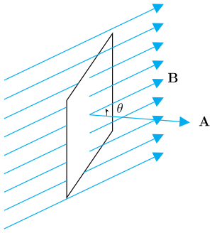
Figure 6.4A plane of surface area A placed in a uniform magnetic field B.

Fig. 6.4 — A plane of surface area A placed in a uniform magnetic field B.

Drawn by us to help you understand the concept clearly, and verified to make sure it's accurate. For exams, practice from your NCERT textbook's own diagram.

The figure shows a flat surface of area $A$ , drawn as a parallelogram, placed inside a uniform magnetic field represented by seven parallel, equally spaced straight lines with arrowheads running diagonally across the frame. The field is the same in magnitude and direction everywhere.

A vector $\mathbf{A}$ (the area vector) is drawn from the plane, pointing to the right along the outward normal to the surface. A bold vector $\mathbf{B}$ (the magnetic field vector) is shown at the upper-right, aligned with the field lines. The angle $\theta$ between the area vector $\mathbf{A}$ and the field vector $\mathbf{B}$ is marked at the plane.

The physical idea is that magnetic flux depends not only on the field strength and area, but also on how the surface is oriented relative to the field. When the plane is tilted, only the component of $\mathbf{B}$ perpendicular to the surface contributes to the flux.

The key formula developed from this figure is:

\Phi_B = \mathbf{B} \cdot \mathbf{A} = B A \cos \theta

where:

$\Phi_B$ is the magnetic flux through the surface (a scalar, SI unit: weber, Wb),
$\mathbf{B}$ is the uniform magnetic field (magnitude $B$ , unit: tesla, T),
$\mathbf{A}$ is the area vector (magnitude $A$ , direction along the outward normal to the surface),
$\theta$ is the angle between $\mathbf{B}$ and $\mathbf{A}$ . …

Figure 6.5Magnetic field Bᵢ at the iᵗʰ area element. dAᵢ represents area vector of the iᵗʰ area element.

Fig. 6.5 — Magnetic field Bᵢ at the iᵗʰ area element. dAᵢ represents area vector of the iᵗʰ area element.

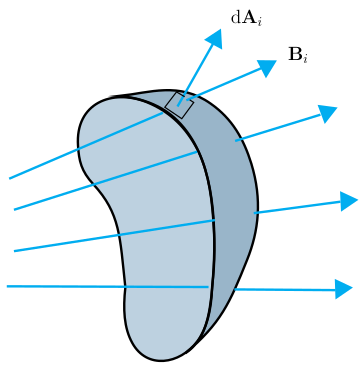
Drawn by us to help you understand the concept clearly, and verified to make sure it's accurate. For exams, practice from your NCERT textbook's own diagram.

The figure illustrates how to calculate magnetic flux through a curved surface placed in a non-uniform magnetic field. It shows a blue, warped 3‑D sheet (the surface) with several parallel blue arrows (the magnetic field lines $\mathbf{B}$ ) passing through it from left to right. The field is not uniform — the arrows have slightly different lengths and directions at different points on the surface.

A small, flat, tilted square (the area element) is highlighted near the top of the surface. Two vectors are drawn at this patch:

$\mathbf{dA}_i$ — the area vector of the $i^\text{th}$ element. It points outward (up‑and‑right) from the surface, perpendicular to the tiny patch. Its magnitude equals the area of the patch.
$\mathbf{B}_i$ — the local magnetic field vector at that same patch. It points to the right, making an angle with $\mathbf{dA}_i$ .

The physical idea is that for a curved surface or a non‑uniform field, we cannot use a single product $BA\cos\theta$ for the whole surface. Instead, we divide the surface into many tiny flat area elements $d\mathbf{A}_i$ , each small enough that the field $\mathbf{B}_i$ is nearly constant over it. The flux through one such element is the dot product $\mathbf{B}_i \cdot d\mathbf{A}_i$ .

The total magnetic flux $\Phi_B$ through the entire curved surface is the sum (integral) of these contributions:

\Phi_B = \sum_{\text{all } i} \mathbf{B}_i \cdot d\mathbf{A}_i

or, in integral form:

\Phi_B = \int \mathbf{B} \cdot d\mathbf{A}

Here:

$\Phi_B$ = magnetic flux (unit: weber, Wb, or T m²)
$\mathbf{B}_i$ = magnetic field vector at the $i^\text{th}$ area element …

Start your 14-day free trial to unlock the full solution →

← Previous · 6.2The Experiments of Faraday and Henry Next · 6.4 →Faraday's Law of Induction