Mathematics · Ch 7 — Applications of Differential Calculus
Asymptotes
Asymptotes
An asymptote for the curve is a straight line which is, informally, "a tangent at infinity" to the curve — the distance between the curve and the line tends to as the point on the curve runs off to infinity. There are three types.
1. Horizontal asymptote (parallel to the -axis). is a horizontal asymptote for if either
2. Vertical asymptote (parallel to the -axis). is a vertical asymptote for if
3. Slant (oblique) asymptote. Occurs when, for a rational function, the numerator's degree is exactly one higher than the denominator's. Found by dividing the numerator by the denominator (long or synthetic division): the quotient (a linear polynomial) is the slant asymptote; the remainder over the denominator vanishes as .
Worked patterns (Examples 7.66–7.68):
- : as , ; as , — so is a vertical asymptote; by symmetry (the curve is unchanged under ), is a horizontal asymptote too, giving the familiar rectangular-hyperbola shape.
- -type expression: numerator degree (2) exceeds denominator degree (1) by exactly one a slant asymptote exists; long division gives the linear quotient directly as the asymptote's equation (the curve approaches this line but never actually touches it). …
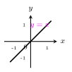
Drawn by us to help you understand the concept clearly, and verified to make sure it's accurate. For exams, practice from your textbook's own diagram.
What this figure shows. Graph of the line y = x, symmetric with respect to the origin. …

Drawn by us to help you understand the concept clearly, and verified to make sure it's accurate. For exams, practice from your textbook's own diagram.
What this figure shows. Graph of the parabola y = x^2, symmetric with respect to the y-axis. …
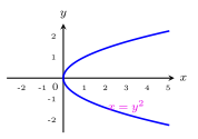
Drawn by us to help you understand the concept clearly, and verified to make sure it's accurate. For exams, practice from your textbook's own diagram.
What this figure shows. Graph of the sideways parabola x = y^2, opening to the right and symmetric with respect to the x …
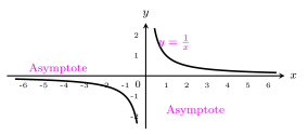
Drawn by us to help you understand the concept clearly, and verified to make sure it's accurate. For exams, practice from your textbook's own diagram.
What this figure shows. Graph of y = 1/x, a rectangular hyperbola with the y-axis (x=0) as vertical asymptote and the x-axis (y=0) as horizontal …
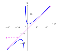
Drawn by us to help you understand the concept clearly, and verified to make sure it's accurate. For exams, practice from your textbook's own diagram.
What this figure shows. Graph of f(x) = (x^2 - 6x + 7)/(x + 5) with its slant (oblique) asymptote y = x - 11; the curve approaches the line but never crosses it. (Axes compressed by …
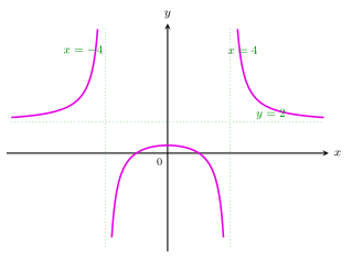
Drawn by us to help you understand the concept clearly, and verified to make sure it's accurate. For exams, practice from your textbook's own diagram.
What this figure shows. Graph of f(x) = (2x^2 - 8)/(x^2 - 16) with vertical asymptotes x = -4 and x = 4 and horizontal asymptote y = 2; the central branch peaks …
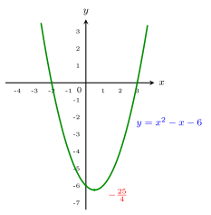
Drawn by us to help you understand the concept clearly, and verified to make sure it's accurate. For exams, practice from your textbook's own diagram.
What this figure shows. Curve sketch of y = x^2 - x - 6 = (x-3)(x+2): x-intercepts (-2,0) and (3,0), y-intercept (0,-6), vertex (local minimum) at (1 …
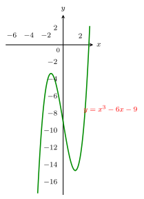
Drawn by us to help you understand the concept clearly, and verified to make sure it's accurate. For exams, practice from your textbook's own diagram.
What this figure shows. Curve sketch of y = x^3 - 6x - 9: x-intercept (3,0), y-intercept (0,-9), local maximum at (-sqrt2, 4sqrt2 - 9) and local minimum at (sqrt2, -4sqrt2 - 9), point of inf …
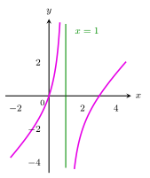
Drawn by us to help you understand the concept clearly, and verified to make sure it's accurate. For exams, practice from your textbook's own diagram.
What this figure shows. Curve sketch of y = (x^2 - 3x)/(x - 1) = x(x-3)/(x-1): passes through the origin and (3,0), with vertical asympto …
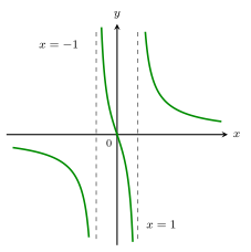
Drawn by us to help you understand the concept clearly, and verified to make sure it's accurate. For exams, practice from your textbook's own diagram.
What this figure shows. Curve sketch of y = 3x/(x^2 - 1): vertical asymptotes x = -1 and x = 1, horizontal asymptote y = 0, point of inflection at the or …