Economics · Ch 10 — The Theory of the Firm under Perfect Competition

Price Elasticity of Supply

10.7

Price Elasticity of Supply

4.7 Price Elasticity of Supply

The price elasticity of supply measures how much the quantity supplied of a good changes when its price changes. It is the supply-side counterpart to the price elasticity of demand you studied earlier.

Definition and Formula

The price elasticity of supply, denoted by $e_S$ , is defined as:

e_S = \frac{\text{Percentage change in quantity supplied}}{\text{Percentage change in price}}

Let $\Delta Q$ be the change in quantity supplied and $\Delta P$ be the change in price. If the original price is $P$ and the original quantity supplied is $Q$ , then:

e_S = \frac{\frac{\Delta Q}{Q} \times 100}{\frac{\Delta P}{P} \times 100} = \frac{\Delta Q}{Q} \times \frac{P}{\Delta P} = \frac{\Delta Q}{\Delta P} \times \frac{P}{Q}

The formula $\frac{\Delta Q}{\Delta P} \times \frac{P}{Q}$ is the most convenient form for calculation. Notice that, like demand elasticity, supply elasticity is independent of the units in which price and quantity are measured — it is a pure number.

A Worked Numerical Example

Consider a perfectly competitive market for cricket balls.

When the price of a cricket ball is ₹10, firms produce 200 balls in total.
When the price rises to ₹30, firms produce 1,000 balls in total.

We can summarise this:

	Price (₹)	Quantity Supplied
Old (1)	$P_1 = 10$	$Q_1 = 200$
New (2)	$P_2 = 30$	$Q_2 = 1000$

Step 1: Calculate the percentage change in quantity supplied.

\text{Percentage change in quantity} = \frac{\Delta Q}{Q_1} \times 100 = \frac{Q_2 - Q_1}{Q_1} \times 100 = \frac{1000 - 200}{200} \times 100 = \frac{800}{200} \times 100 = 400\%

Step 2: Calculate the percentage change in price.

\text{Percentage change in price} = \frac{\Delta P}{P_1} \times 100 = \frac{P_2 - P_1}{P_1} \times 100 = \frac{30 - 10}{10} \times 100 = \frac{20}{10} \times 100 = 200\%

Step 3: Compute the price elasticity of supply.

e_S = \frac{400\%}{200\%} = 2

An elasticity of 2 means that for every 1% increase in price, the quantity supplied increases by 2%. Supply is quite responsive to price changes in this example.

The Sign of Elasticity

When the supply curve is vertical, quantity supplied does not change at all when price changes. In that case, $\Delta Q = 0$ , so $e_S = 0$ . Supply is perfectly inelastic.

For any positively sloped supply curve, a rise in price leads to a rise in quantity supplied. Both $\Delta Q$ and $\Delta P$ are positive, so the elasticity $e_S$ is always positive. This is a key difference from demand elasticity, which is negative.

Watch out

A common mistake is to treat supply elasticity as negative. Remember: supply curves slope upward, so price and quantity move in the same direction. The elasticity of supply is always a positive number (or zero for a vertical supply curve).

Note

The Geometric Method

There is a neat geometric way to read the price elasticity of supply at any point on a straight-line supply curve, with no arithmetic at all. Take any point $S$ on the supply curve and drop a perpendicular from it to the quantity-axis, meeting that axis at $q_0$ . Next, extend the supply curve (if it does not already reach the axis) until it meets the quantity-axis; call this point $M$ . The price elasticity of supply at $S$ is then simply the ratio $e_S = Mq_0 / Oq_0$ , where $O$ is the origin. Where $M$ falls relative to the origin — shown in the three panels of the figure below — tells us at a glance whether the elasticity is greater than, equal to, or less than one.

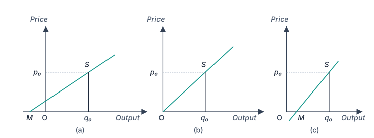
Figure 4.14Price Elasticity Associated with Straight Line Supply Curves. In panel (a), price elasticity (e_s) at S is greater than 1. In panel (b), price elasticity (e_s) at S is equal to 1. In panel (c), price elasticity (e_s) at S is less than 1.

Fig. 4.14 — Price Elasticity Associated with Straight Line Supply Curves. In panel (a), price elasticity (e_s) at S is greater than 1. In panel (b), price elasticity (e_s) at S is equal to 1. In panel (c), price elasticity (e_s) at S is less than 1.

Drawn by us to help you understand the concept clearly, and verified to make sure it's accurate. For exams, practice from your textbook's own diagram.

The figure shows three straight-line supply curves, one per panel (a), (b) and (c). Every panel has its own pair of axes: price on the vertical axis and output on the horizontal axis. On each line a point $S$ is marked, at output $q_0$ and price $p_0$ . What differs across the panels is where the extended supply line meets the output axis — the point labelled $M$ — and that is exactly what decides the price elasticity of supply.

The geometric measure the textbook develops with this figure is:

e_s = \frac{Mq_0}{Oq_0}

Here $O$ is the origin, $q_0$ is the output at the chosen point $S$ , and $M$ is the point where the straight supply line (extended if necessary) cuts the output axis. $Mq_0$ is the distance from $M$ to $q_0$ along that axis, and $Oq_0$ is the distance from the origin to $q_0$ .

Why this works: along a straight line through $M$ , price rises from $0$ (at $M$ ) to $p_0$ (at output $q_0$ ), so $\frac{\Delta q}{\Delta p} = \frac{Mq_0}{p_0}$ . Substituting into the definition $e_s = \frac{p_0}{q_0}\cdot\frac{\Delta q}{\Delta p}$ gives $e_s = \frac{p_0}{q_0}\cdot\frac{Mq_0}{p_0} = \frac{Mq_0}{Oq_0}$ , since $Oq_0 = q_0$ .

Panel (a): $e_s > 1$ . The line cuts the output axis at $M$ to the left of the origin (equivalently, it meets the price axis at a positive price). Then $Mq_0 > Oq_0$ , so $e_s > 1$ — and since $S$ can be any point on the line, elasticity exceeds 1 at every point on such a supply curve.
Panel (b): $e_s = 1$ . The line passes through the origin — imagine $M$ has coincided with $O$ , so $Mq_0 = Oq_0$ and $e_s = 1$ . Any straight-line supply curve through the origin has unit price elasticity at every point, whatever its slope.
Panel (c): $e_s < 1$ . The line cuts the output axis at $M$ between $O$ and $q_0$ (it would meet the price axis at a negative price, which is why the drawn line continues a little below the output axis). Then $Mq_0 < Oq_0$ , so $e_s < 1$ at every point on the line. …

Case 1: Supply curve cuts the price-axis (positive intercept on the price-axis).

In panel (a) of Figure 4.14, the supply curve meets the price-axis at a positive value. When extended backward, it cuts the quantity-axis at a point $M$ that lies to the left of the origin (in the negative range of the quantity-axis). The distance $Mq_0$ is therefore greater than $Oq_0$ . Hence:

e_S = \frac{Mq_0}{Oq_0} > 1

Supply is elastic at every point on such a supply curve.

Case 2: Supply curve passes through the origin.

In panel (b), the supply curve goes through the origin. The point $M$ coincides with the origin $O$ . Therefore $Mq_0 = Oq_0$ , and:

e_S = \frac{Oq_0}{Oq_0} = 1

Supply has unit elasticity at every point on a straight-line supply curve that passes through the origin.

Case 3: Supply curve cuts the quantity-axis (positive intercept on the quantity-axis).

In panel (c), the supply curve meets the quantity-axis at a point $M$ that lies to the right of the origin (in the positive range). The distance $Mq_0$ is now less than $Oq_0$ . Hence:

$e_S = \frac{Mq_0}{Oq_0} < 1$ …

Start your 14-day free trial to unlock the full solution →

← Previous · 10.6Market Supply Curve Next · key-concepts →Key Concepts