Economics · Ch 8 — Theory of Consumer Behaviour

Elasticity along a Linear Demand Curve

8.6.1

Elasticity along a Linear Demand Curve

Elasticity Changes Along a Linear Demand Curve

A linear demand curve is written as $q = a - bp$ , where $a$ and $b$ are positive constants. The slope of this curve is constant: for every one-unit change in price, quantity demanded changes by $-b$ units. That is, $\frac{\Delta q}{\Delta p} = -b$ at every point.

But price elasticity of demand is not the same as slope. Elasticity is defined as:

e_D = \frac{\Delta q}{\Delta p} \times \frac{p}{q}

Substituting the constant slope $-b$ gives:

e_D = -b \times \frac{p}{q}

Now replace $q$ with $a - bp$ :

e_D = -\frac{bp}{a - bp}

This is equation (2.17) in the textbook. The negative sign is often ignored when we talk about the absolute value $|e_D|$ , but the formula itself carries the sign because demand curves slope downward.

The key insight is that even though the slope is fixed, the ratio $\frac{p}{q}$ changes as you move along the line. So elasticity varies from one point to another.

Where Elasticity Takes Specific Values

At $p = 0$ (where the demand curve meets the horizontal axis), the numerator $bp$ is zero, so $e_D = 0$ . Demand is perfectly inelastic at that point.
At $q = 0$ (where the demand curve meets the vertical axis), the denominator $a - bp$ becomes zero, so $e_D$ tends to infinity. Demand is perfectly elastic at that point.
At the midpoint of the demand curve, price equals $\frac{a}{2b}$ . Plugging this into the formula gives $e_D = -1$ . The absolute value is exactly 1 — unitary elastic.
For any price between $0$ and $\frac{a}{2b}$ , the elasticity is less than 1 in absolute value (inelastic region).
For any price greater than $\frac{a}{2b}$ (but below the vertical intercept), elasticity is greater than 1 (elastic region).

Watch out

A common mistake is to think that a linear demand curve has constant elasticity. It does not — only the slope is constant. Elasticity changes continuously along the line.

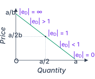
The textbook illustrates this with Figure 2.19, which shows a downward-sloping straight line. At the top (near the vertical axis), the demand curve is steep relative to the price-quantity ratio, so elasticity is high. At the bottom (near the horizontal axis), it is flat relative to that ratio, so elasticity is low.

Figure 2.19Elasticity along a Linear Demand Curve. Price elasticity of demand is different at different points on the linear demand curve.

Fig. 2.19 — Elasticity along a Linear Demand Curve. Price elasticity of demand is different at different points on the linear demand curve.

Drawn by us to help you understand the concept clearly, and verified to make sure it's accurate. For exams, practice from your textbook's own diagram.

Figure 2.19 is a simple two-axis graph with a single straight line sloping downward from the vertical axis to the horizontal axis. The vertical axis is labelled Price, and the horizontal axis is labelled Quantity. The demand curve itself is the line $q = a - bp$ , so it hits the price axis at $a/b$ (when $q=0$ ) and the quantity axis at $a$ (when $p=0$ ).

Five specific points are marked along this line, each with a label showing the value of $|e_D|$ at that location.

At the very top, where the demand curve meets the price axis, the label reads $|e_D| = \infty$ . This is the point where price is highest and quantity demanded is zero. At the very bottom, where the demand curve meets the quantity axis, the label reads $|e_D| = 0$ . This is the point where price is zero and quantity demanded is at its maximum.

Exactly halfway along the line — at the midpoint — a dashed horizontal guide line extends left to the price axis at $p = a/2b$ , and a dashed vertical guide line drops down to the quantity axis at $q = a/2$ . At this intersection, the label reads $|e_D| = 1$ .

On the upper half of the demand curve, between the top and the midpoint, the label says $|e_D| > 1$ . On the lower half, between the midpoint and the bottom, the label says $|e_D| < 1$ .

Important

The central lesson of this figure is that elasticity is not constant along a straight-line demand curve. Even though the slope ( $-b$ ) is the same everywhere, elasticity depends on the ratio $p/q$ , which changes as you move along the line. The midpoint is the only place where the percentage change in quantity exactly matches the percentage change in price. …

Constant Elasticity Demand Curves

Not all demand curves have varying elasticity. Some special shapes keep elasticity fixed.

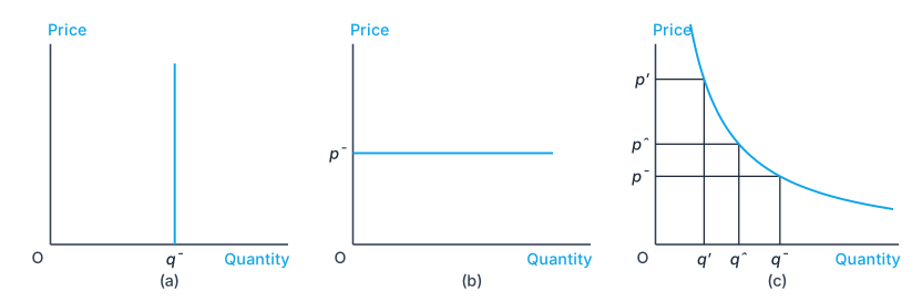
Perfectly inelastic demand (vertical line): Figure 2.20(a) shows a vertical demand curve at quantity $\bar{q}$ . No matter what the price, quantity demanded stays the same. A price change causes zero change in quantity, so $|e_D| = 0$ at every point. This is a vertical straight line.

Perfectly elastic demand (horizontal line): Figure 2.20(b) shows a horizontal demand curve at price $\bar{P}$ . At any price above $\bar{P}$ , quantity demanded drops to zero; at any price below, it becomes infinite (in theory). The elasticity is infinite at every point. This is a horizontal straight line.

Unitary elastic demand (rectangular hyperbola): Figure 2.20(c) depicts a demand curve shaped like a rectangular hyperbola. Its special property is that a percentage change in price always leads to an equal percentage change in quantity in the opposite direction, so $|e_D| = 1$ at every point. The equation of such a curve is $q = \frac{k}{p}$ for some constant $k$ , so total expenditure $p \times q$ remains constant along the curve.

Important

The three constant-elasticity cases — vertical (zero), horizontal (infinite), and rectangular hyperbola (unitary) — are the only demand curves where elasticity does not change with price.

Figure 2.20Constant Elasticity Demand Curves. Elasticity of demand at all points along the vertical demand curve, as shown in panel (a), is 0. Elasticity of demand at all point along the horizontal demand curve, as shown in panel (b) is ∞. Elasticity at all points on the demand curve in panel (c) is 1.

Fig. 2.20 — Constant Elasticity Demand Curves. Elasticity of demand at all points along the vertical demand curve, as shown in panel (a), is 0. Elasticity of demand at all point along the horizontal demand curve, as shown in panel (b) is ∞. Elasticity at all points on the demand curve in panel (c) is 1.

Drawn by us to help you understand the concept clearly, and verified to make sure it's accurate. For exams, practice from your textbook's own diagram.

Figure 2.20 places three demand curves side by side, each in its own panel labelled (a), (b), and (c). In every panel, price is measured on the vertical axis and quantity on the horizontal axis. The purpose is to show three special cases where the price elasticity of demand is the same at every point on the curve — something that never happens on a straight-line demand curve.

Panel (a) shows a vertical straight line at a fixed quantity, labelled $\bar{q}$ . No matter what price is chosen on the vertical axis, the quantity demanded stays at $\bar{q}$ . Because a change in price produces zero change in quantity, the elasticity $|e_D|$ is 0 at every point. This is called a perfectly inelastic demand curve.

Panel (b) shows a horizontal straight line at a fixed price, labelled $\bar{P}$ . The quantity demanded can be any value along the horizontal axis, but only at price $\bar{P}$ . If the price rises even slightly above $\bar{P}$ , quantity demanded drops to zero; if it falls below $\bar{P}$ , quantity demanded becomes infinite (in theory). The percentage change in quantity for any tiny price change is effectively infinite, so $|e_D| = \infty$ at every point. This is a perfectly elastic demand curve.

Panel (c) shows a curve that bends downward from left to right, shaped like a rectangular hyperbola. Three specific points are marked on this curve, each connected by solid-sided rectangles to the axes. At the highest price $p'$ , the rectangle runs down to quantity $q'$ ; at the middle price $\hat{p}$ , it runs down to quantity $\hat{q}$ ; at the lowest price $\bar{p}$ , it runs down to quantity $\bar{q}$ . The key property of a rectangular hyperbola is that the product $p \times q$ is constant at every point. That means a 1% rise in price is always matched by a 1% fall in quantity, so $|e_D| = 1$ everywhere. This is called a unitary elastic demand curve. …

Geometric Measure of Elasticity on a Straight Line

Geometric measure of elasticity along a linear demand curve: a straight demand line from B on the price axis to A on the quantity axis, with prices p¹ and p⁰, quantities q¹ and q⁰, points E and D on the line and corner C forming the similar triangles that give elasticity as the segment ratio DA/DB.

Drawn by us to help you understand the concept clearly, and verified to make sure it's accurate. For exams, practice from your textbook's own diagram.

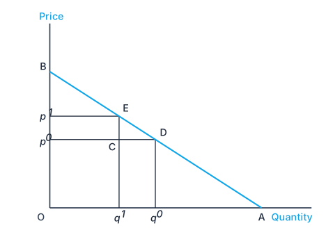
The elasticity of a straight-line demand curve at any point equals the ratio of the lower segment to the upper segment of the line at that point. A price change from p⁰ to p¹ moves the chosen point from D to E; because triangles ECD, Bp⁰D and BOA are similar, the ratios collapse to $e_D = DA/DB$ — so elasticity is 1 at the midpoint of …

Note

Geometric Measure of Elasticity along a Linear Demand Curve

There is a neat geometric shortcut for the elasticity at any point on a linear demand curve, without using the formula: the elasticity at a point equals the ratio of the lower segment of the demand curve to the upper segment at that point.

To see why, take a straight-line demand curve $q = a - bp$ . Let the initial price be $p_0$ and quantity $q_0$ ; raise the price to $p_1$ so quantity falls to $q_1$ . Then $\Delta q = q_1 - q_0$ is the horizontal distance CD and $\Delta p = p_1 - p_0$ is the vertical distance CE. From the elasticity formula,

$e_D = \frac{\Delta q}{\Delta p} \times \frac{p_0}{q_0} = \frac{CD}{CE} \times \frac{Op_0}{Oq_0}$

Triangles ECD and $Bp_0D$ are similar, so $\frac{CD}{CE} = \frac{p_0 D}{p_0 B}$ . Since $p_0 D = Oq_0$ , this gives $\frac{CD}{CE} = \frac{Oq_0}{p_0 B}$ , and substituting back,

$e_D = \frac{Oq_0}{p_0 B} \times \frac{Op_0}{Oq_0} = \frac{Op_0}{p_0 B}$ …

Start your 14-day free trial to unlock the full solution →

← Previous · 8.6Elasticity of Demand Next · 8.6.2 →Factors Determining Price Elasticity of Demand for a Good