Physics · Ch 7 — Alternating Current

AC Voltage Applied to an Inductor

7.4

AC Voltage Applied to an Inductor

Why an Inductor Behaves Differently from a Resistor in AC

When an AC voltage is applied to a pure inductor (one with negligible resistance), the inductor does not oppose current in the same way a resistor does. Instead, it opposes changes in current through self-induced emf. This leads to a phase difference between voltage and current — a key concept in AC circuits.

Deriving the Current in a Purely Inductive AC Circuit

Consider an AC source connected to an inductor of inductance $L$ . The source voltage is:

v = v_m \sin(\omega t)

where $v_m$ is the peak voltage and $\omega$ is the angular frequency.

Applying Kirchhoff's loop rule, the sum of potential differences around the loop is zero. The only emf in the circuit is the source voltage $v$ and the self-induced emf in the inductor, which is $-L \frac{di}{dt}$ (the negative sign comes from Lenz's law). Thus:

v - L \frac{di}{dt} = 0

Rearranging gives the differential equation for the current:

\frac{di}{dt} = \frac{v}{L} = \frac{v_m}{L} \sin(\omega t)

This tells us that the slope of the current ( $di/dt$ ) varies sinusoidally with the same phase as the voltage.

To find $i(t)$ , integrate both sides with respect to time:

i(t) = \int \frac{di}{dt} \, dt = \int \frac{v_m}{L} \sin(\omega t) \, dt

i(t) = -\frac{v_m}{\omega L} \cos(\omega t) + \text{constant}

The integration constant represents any steady (DC) component of current. Since the AC source oscillates symmetrically about zero, the current also oscillates symmetrically — so the constant is zero.

Using the trigonometric identity $-\cos(\omega t) = \sin\left(\omega t - \frac{\pi}{2}\right)$ , we write:

i(t) = i_m \sin\left(\omega t - \frac{\pi}{2}\right)

where the current amplitude is:

i_m = \frac{v_m}{\omega L}

Inductive Reactance

The quantity $\omega L$ plays the role of "resistance" in this circuit. It is called inductive reactance, denoted by $X_L$ :

X_L = \omega L = 2\pi f L

$X_L$ has the same SI unit as resistance: ohm ( $\Omega$ ).
It limits the current in a purely inductive circuit just as resistance does in a resistive circuit.
$X_L$ is directly proportional to both the inductance $L$ and the frequency $f$ of the AC source.

The current amplitude can then be written as:

i_m = \frac{v_m}{X_L}

Phase Relationship: Current Lags Voltage

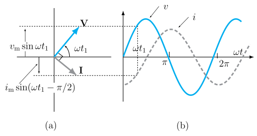
Comparing the voltage $v = v_m \sin(\omega t)$ and the current $i = i_m \sin(\omega t - \pi/2)$ , we see that the current is shifted by $-\pi/2$ radians (or $-90^\circ$ ) relative to the voltage.

Current lags behind the voltage by $\pi/2$ (one-quarter of a cycle).
In phasor terms, the current phasor $\mathbf{I}$ is $\pi/2$ behind the voltage phasor $\mathbf{V}$ when rotated counterclockwise at angular frequency $\omega$ .

Power in a Purely Inductive Circuit

Instantaneous power supplied to the inductor is: …

Figure 7.5An ac source connected to an inductor.

Fig. 7.5 — An ac source connected to an inductor.

Drawn by us to help you understand the concept clearly, and verified to make sure it's accurate. For exams, practice from your textbook's own diagram.

What the Figure Shows

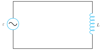
The figure is a simple series circuit diagram with two components connected by straight top and bottom conductors:

Left side: An AC voltage source, drawn as a circle containing a wavy line (∼), labelled with the symbol ε (the source emf).
Right side: An inductor, drawn as a coil of several loops (like a solenoid), labelled L (its self-inductance).

The source and inductor are joined in a single rectangular loop — there is no resistor in the circuit. This is a purely inductive AC circuit.

Physical Idea Taught

The figure illustrates the application of Kirchhoff’s loop rule to an AC circuit containing only an inductor. The key physics is:

The source voltage is sinusoidal:

v = v_m \sin(\omega t)

where $v_m$ is the peak voltage and $\omega$ is the angular frequency.

The inductor opposes changes in current via self-induced emf (Faraday’s law). The loop rule gives:

v - L \frac{di}{dt} = 0 \quad \Rightarrow \quad \frac{di}{dt} = \frac{v}{L} = \frac{v_m}{L} \sin(\omega t)

Integrating this yields the current:

i = i_m \sin\left(\omega t - \frac{\pi}{2}\right)

where the current amplitude is:

i_m = \frac{v_m}{\omega L}

Key Formulas Developed from This Figure

Inductive reactance (the opposition to current offered by the inductor):

X_L = \omega L

$X_L$ has units of ohms (Ω).
It depends on both the inductance $L$ and the frequency $\omega$ (or $f$ , since $\omega = 2\pi f$ ).

Current amplitude in terms of reactance:

i_m = \frac{v_m}{X_L}

Phase relationship: The current lags the voltage by $\frac{\pi}{2}$ (one-quarter cycle). This is seen directly from the sine functions: voltage is $\sin(\omega t)$ , current is $\sin(\omega t - \pi/2)$ .
Instantaneous power supplied to the inductor:

p_L = v i = - \frac{v_m i_m}{2} \sin(2\omega t)

The average power over a complete cycle is zero — the inductor stores and releases energy but does not dissipate it. …

Figure 7.6(a) A Phasor diagram for the circuit in Fig. 7.5. (b) Graph of v and i versus ωt.

Fig. 7.6 — (a) A Phasor diagram for the circuit in Fig. 7.5. (b) Graph of v and i versus ωt.

Drawn by us to help you understand the concept clearly, and verified to make sure it's accurate. For exams, practice from your textbook's own diagram.

What Figure 7.6 Shows

The figure has two panels that together illustrate the phase relationship between voltage and current in a purely inductive AC circuit (the circuit of Fig. 7.5, where an AC source is connected to an ideal inductor with zero resistance).

Panel (a): Phasor Diagram

This is a snapshot at a particular instant $t_1$ . Two rotating arrows (phasors) are drawn:

Voltage phasor $V$ : Points up-and-right, making an angle $\omega t_1$ with the horizontal. Its vertical projection is labelled $v_m \sin \omega t_1$ , which is the instantaneous voltage at that instant.
Current phasor $I$ : Points down-and-right, below the horizontal. It is drawn a quarter-turn clockwise behind $V$ , meaning it lags by $\pi/2$ radians (90°). Its vertical projection is labelled $i_m \sin(\omega t_1 - \pi/2)$ , which is the instantaneous current at that instant.

The key visual: the current phasor is $\pi/2$ behind the voltage phasor when both rotate counterclockwise.

Panel (b): Graph of $v$ and $i$ versus $\omega t$

The horizontal axis is $\omega t$ (in radians), with ticks at $\omega t_1$ , $\pi$ , and $2\pi$ . Two curves are plotted:

Voltage $v$ (solid curve): A sine wave $v = v_m \sin \omega t$ .
Current $i$ (dashed curve): A sine wave $i = i_m \sin(\omega t - \pi/2)$ , shifted a quarter-period to the right (later in time) relative to the voltage.

The graph shows that the voltage reaches its peak before the current does — the current lags the voltage by exactly one-quarter of a cycle.

Physical Idea Taught

In a pure inductor, the current lags the applied voltage by $\pi/2$ (90°). This happens because the inductor opposes changes in current (Lenz’s law). When the voltage is at its maximum, the current is still zero and just starting to rise; when the current reaches its maximum a quarter-cycle later, the voltage has already dropped to zero.

Key Formulas Developed with This Figure

From the textbook derivation (Eqs. 7.11–7.14), the figure directly supports:

v = v_m \sin \omega t

i = i_m \sin\left(\omega t - \frac{\pi}{2}\right)

where:

$v_m$ = peak voltage (amplitude)
$i_m = \frac{v_m}{\omega L}$ = peak current (amplitude)
$\omega$ = angular frequency of the source ( $\omega = 2\pi f$ )
$L$ = self-inductance of the inductor …

Start your 14-day free trial to unlock the full solution →

← Previous · 7.3Representation of AC Current and Voltage by Rotating Vectors — Phasors Next · 7.4 →Example 7.2 — A pure inductor of 25.0mH is connected to a source of 220V. Find the i…

AC Voltage Applied to an Inductor