Physics · Ch 6 — System of Particles and Rotational Motion
Centre of Mass
Centre of Mass
6.2 Centre of Mass
The Core Idea
When we study the motion of a system of particles — whether it's two atoms or a spinning cricket bat — we quickly realise that tracking every single particle is impractical. The centre of mass is the single point that behaves as if the entire mass of the system were concentrated there, and as if all external forces acted at that point. For a rigid body undergoing pure translation, every particle moves exactly as the centre of mass moves. For more complex motion that includes rotation, the centre of mass still follows a simple translational path, while the body rotates about it.
Two-Particle System Along a Line
Consider two particles of masses and lying on the -axis. Let their positions be and measured from some origin O. The centre of mass of this two-particle system is the point C whose coordinate is given by
This is a mass-weighted average of the positions. If the two masses are equal (), then
so the centre of mass lies exactly midway between the two particles.
The centre of mass is not necessarily the geometric centre — it is pulled toward the heavier particle. Only when masses are equal does it coincide with the midpoint.
Generalisation to Particles on a Line
For particles of masses placed along the -axis at positions , the centre of mass coordinate is
The denominator is the total mass . Using summation notation,
Centre of Mass in a Plane
For three particles not lying on a straight line, we set up and axes in their plane. Let the particles have masses and coordinates . The centre of mass is at where
If all three masses are equal (), then
These are precisely the coordinates of the centroid of the triangle formed by the three particles. For equal masses, the centre of mass coincides with the centroid.
Centre of Mass in Space: The Vector Form
For particles distributed in three-dimensional space, with the th particle of mass at , the centre of mass coordinates are
where is the total mass.
These three scalar equations combine elegantly into a single vector equation. Let be the position vector of the th particle, and let be the position vector of the centre of mass. Then
If we choose the centre of mass itself as the origin of our coordinate system, then , which gives
This condition is often useful in derivations.
Continuous Mass Distribution
A rigid body is a system of closely packed particles — so many that summing over individual atoms is impossible. Instead, we treat the body as a continuous distribution of mass.
We divide the body into small elements of mass , each located approximately at . The centre of mass coordinates are approximately
As we take larger and each smaller, these approximations become exact. The sums become integrals:
and similarly for and . The exact centre of mass coordinates are therefore
The vector form is
If the centre of mass is taken as the origin, then , which implies
or equivalently
Symmetry and the Centre of Mass of Homogeneous Bodies
For homogeneous bodies (uniform mass distribution) of regular shape — rings, discs, spheres, rods — the centre of mass lies at the geometric centre. This follows from reflection symmetry. …
Drawn by us to help you understand the concept clearly, and verified to make sure it's accurate. For exams, practice from your NCERT textbook's own diagram.
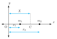
The figure shows a straight horizontal line — the x-axis — with two points labelled and placed at positions and respectively. A third point, labelled C (the centre of mass), lies somewhere between them at coordinate . A dashed vertical line drops from C down to the axis, marking its location clearly. The origin O is at the left end of the axis, and a vertical y-axis is drawn through O, though the figure is essentially one-dimensional.
The physical idea is simple: if you have two masses on a line, there is a single point — the centre of mass — that behaves as if the entire mass of the system were concentrated there. For two particles, this point always lies on the line joining them, closer to the heavier mass. The figure makes this concrete by placing and at known coordinates and showing C at the weighted average of their positions.
The textbook uses this diagram to derive the formula for the centre of mass of a two-particle system. The key step is to require that the total torque about the centre of mass is zero — or equivalently, that the centre of mass is the point where the weighted sum of distances from any reference point equals the total mass times the distance to that reference point. From the figure, with the origin at O, the definition gives:
Here and are the masses of the two particles, and are their positions on the x-axis, and is the x-coordinate of the centre of mass C. The denominator is the total mass of the system.
The centre of mass is the mass-weighted average position of the particles. For two particles on a line, it always lies between them — exactly at the midpoint only if the masses are equal, and closer to the heavier mass otherwise.
If you choose the origin at the centre of mass itself (so ), the formula rearranges to , which says that the two particles balance each other about that point — a direct visual takeaway from the figure: the dashed line at C is the balance point. …
Drawn by us to help you understand the concept clearly, and verified to make sure it's accurate. For exams, practice from your NCERT textbook's own diagram.
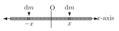
The figure shows a thin rod placed along the x-axis with its centre at the origin O. The rod itself is drawn as a dashed line, indicating it is a continuous object, not a collection of discrete particles. Two small mass elements, each labelled , are marked at symmetric positions: one at and one at . The entire rod extends from to , so its total length is .
The physical idea is straightforward: to find the centre of mass of a continuous object, you cannot sum over individual particles because there are infinitely many. Instead, you imagine cutting the rod into infinitesimally small pieces of mass , each located at some coordinate . The centre of mass is then the weighted average of all these positions, where the weight is the mass of each piece. The symmetry of the figure — two equal mass elements at opposite positions — hints that the centre of mass must lie at the origin. But the textbook uses this setup to derive the general formula.
The key formula developed from this figure is the centre of mass of a continuous body:
Here, is the total mass of the rod, is the position coordinate of a mass element , and the integral runs over the entire length of the rod. For the thin rod, the mass per unit length is constant, so . Substituting this into the integral gives:
The integral of over symmetric limits is zero because the positive and negative contributions cancel exactly. Hence , confirming that the centre of mass of a uniform rod is at its geometric centre. …