Economics · Ch 2 — National Income Accounting

Income Method

2.2.3

Income Method

The Income Method: Measuring GDP by Factor Payments

The third way to measure GDP is the income method. The core idea is simple: every rupee spent on final goods (which we measure in the expenditure method) eventually becomes someone's income. When a firm sells its output, the revenue it earns is not kept entirely as profit — it is distributed to the factors of production that helped create that output.

These factor payments are:

Wages and salaries (paid to labour)
Rent (paid for the use of land)
Interest (paid for the use of capital)
Profit (the residual that goes to the entrepreneur)

If we add up all these incomes earned by all households in the economy during a year, we get the same total as the value of all final goods and services produced — that is, the GDP.

The Formal Identity

Let the economy have $M$ households. For the $i$ -th household in a given year:

$W_i$ = wages and salaries received
$P_i$ = gross profits received
$In_i$ = interest payments received
$R_i$ = rent received

Then, summing across all households:

\text{GDP} \equiv \sum_{i=1}^{M} W_i \;+\; \sum_{i=1}^{M} P_i \;+\; \sum_{i=1}^{M} In_i \;+\; \sum_{i=1}^{M} R_i

We can write this more compactly as:

\text{GDP} \equiv W + P + In + R \qquad(2.5)

where $W$ , $P$ , $In$ , and $R$ are the economy-wide totals of wages, profits, interest, and rent respectively.

Important

This identity is not an approximation — it is an accounting identity. It must hold because every rupee of value added by a firm is either paid to a factor of production or kept as profit (which is itself a factor payment to the entrepreneur).

The Three Methods Are Equivalent

The textbook now brings together all three methods into one powerful identity. From equation (2.2) we had the product method, from (2.4) the expenditure method, and from (2.5) the income method. Together:

\text{GDP} \equiv \sum_{i=1}^{N} GVA_i \equiv C + I + G + X - M \equiv W + P + In + R \qquad(2.6)

Note

In identity (2.6), the symbol $I$ stands for total investment — both planned and unplanned. Unplanned investment (inventory accumulation or depletion) is automatically captured because the expenditure method measures what was actually spent, not what firms intended to spend.

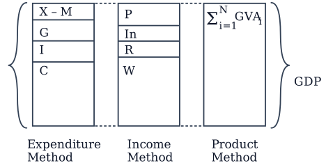
This equivalence is captured in a single diagram (Figure 2.2 in the textbook). The figure sets three columns of boxes side by side and joins them with a large bracket on each side, labelling the whole bracketed group GDP:

Expenditure Method: a column of component boxes — $X - M$ (net exports), $G$ (government expenditure), $I$ (investment) and $C$ (consumption) — that together make up final expenditure.
Income Method: a column of component boxes — $P$ (profit), $In$ (interest), $R$ (rent) and $W$ (wages) — the factor incomes.
Product Method: a single box, $\sum_{i=1}^{N} GVA_i$ , the sum of the gross value added of all firms.

Because the three columns are bracketed together and set equal to GDP, the figure shows at a glance that summing the expenditure components, the income components, or the value added of every firm each arrives at the same total.

Figure 2.2Diagrammatic representation of GDP by the three methods: three bracketed columns of stacked boxes — the expenditure components X − M, G, I and C, the factor incomes P, In, R and W, and a single box summing the gross value added of all firms — jointly labelled GDP

Fig. 2.2 — Diagrammatic representation of GDP by the three methods: three bracketed columns of stacked boxes — the expenditure components X − M, G, I and C, the factor incomes P, In, R and W, and a single box summing the gross value added of all firms — jointly labelled GDP

Drawn by us to help you understand the concept clearly, and verified to make sure it's accurate. For exams, practice from your NCERT textbook's own diagram.

Figure 2.2 sets three columns of boxes side by side and encloses the whole group in a large curly bracket on each side, with a single label — GDP — written against the right bracket. Short dashed lines join the columns at their top and bottom edges, signalling that all three columns span exactly the same total height. There are no arrows: the figure is a statement of equality, not a flow chart.

The Expenditure Method column stacks the components of final expenditure top to bottom: $X - M$ (net exports), $G$ (government expenditure), $I$ (investment) and $C$ (consumption). The $C$ box is drawn noticeably tallest — consumption is the largest expenditure component — while $X - M$ is the thinnest sliver at the top.
The Income Method column stacks the factor incomes: $P$ (profit), $In$ (interest), $R$ (rent) and $W$ (wages), with the $W$ box the tallest.
The Product Method column is one single tall box carrying the summation $\sum_{i=1}^{N} GVA_i$ — the gross value added of every firm in the economy added together. …

A Worked Numerical Example

The textbook gives a simple two-firm economy to demonstrate that all three methods yield the same GDP. Let us walk through it carefully.

The setup:

Firm A grows cotton. It uses no raw material (intermediate goods) and sells its entire output of cotton worth Rs 50 to Firm B.
Firm B uses this cotton as raw material to produce cloth. It sells the finished cloth to consumers for Rs 200.

Method 1: Product (Value Added) Method

Value added = Sales − Cost of intermediate goods.

Firm A: $VA_A = 50 - 0 = 50$
Firm B: $VA_B = 200 - 50 = 150$

\text{GDP} = VA_A + VA_B = 50 + 150 = 200

Method 2: Expenditure Method

Here, the only final good is the cloth sold to consumers. The cotton sold by A to B is an intermediate good — it is not counted in final expenditure.

\text{GDP} = \text{Final expenditure on cloth} = 200

Method 3: Income Method

Now we need to see how the Rs 200 of value added gets distributed as factor incomes.

Firm A receives Rs 50 from selling cotton. It pays Rs 20 as wages to its workers and keeps the remaining Rs 30 as profit.
Firm B receives Rs 200 from selling cloth. It pays Rs 60 as wages and keeps Rs 90 as profit.

Table 2.3: Distributions of factor incomes of firms A and B

Factor Income	Firm A	Firm B
Wages	20	60
Profits	30	90

Start your 14-day free trial to unlock the full solution →

← Previous · 2.2.2Expenditure Method Next · 2.2.4 →Factor Cost, Basic Prices and Market Prices