Business Mathematics and Statistics · Ch 3 — Integral Calculus – II (Area under curves; Application of Integration in Economics and Commerce)
Consumer's Surplus and Producer's Surplus
Consumer's Surplus and Producer's Surplus
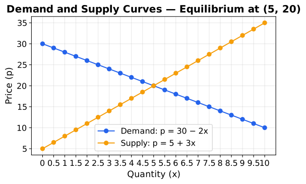
Equilibrium
Given a demand function (price falls as quantity rises) and a supply function (price rises as quantity rises), the equilibrium point is where they meet: .
Consumer's Surplus
Consumer's Surplus (CS) measures the extra amount consumers WOULD have been willing to pay, above what they actually paid at the equilibrium price, for every unit up to :
Producer's Surplus
Producer's Surplus (PS) measures the extra amount producers actually RECEIVED, above the minimum they would have accepted, for every unit up to :
CS uses (area under demand) minus (rectangle); PS uses (rectangle) minus (area under supply) — never the other way round …
, where is the demand function and is the m …
, where is the supply function and is the m …