Mathematics · Ch 11 — Probability Distributions
Random Variable
Random Variable
Definition 11.1 (Random variable). A random variable is a function defined on a sample space into the real numbers , such that the inverse image of every point, subset or interval of is an event in — i.e. a set to which the underlying experiment already assigns a probability.
Notation: capital letters denote random variables (the function itself); the corresponding small letters denote the possible values the random variable can take. Formally , and for a sample point , is the real number assigned to it. The range set (or support) of is — the collection of values actually takes.
Inverse image. If is a value of , its inverse image is the set of all sample points mapping to — and this set is always an event of , so it has a well-defined probability. This is the mechanism that lets us talk about "the probability that equals ": it is really the probability of the underlying event .
Worked illustrations.
- Coin toss. . Let = number of heads: . So is a random variable taking the values and , and e.g. .
- Two coins (finding an inverse image). , number of tails. Then ; takes the values with sample points in their inverse images respectively (total , matching ).
- Two dice. has ordered pairs , ; takes the values , with the familiar triangular counts (summing to ). …
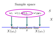
Drawn by us to help you understand the concept clearly, and verified to make sure it's accurate. For exams, practice from your textbook's own diagram.
What this figure shows. A random variable maps sample points of the sample space to points on the real line (the inverse image of a value is an …
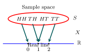
Drawn by us to help you understand the concept clearly, and verified to make sure it's accurate. For exams, practice from your textbook's own diagram.
What this figure shows. The mapping for the number of tails when two coins are tossed: , , , …
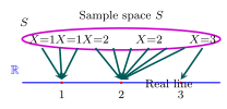
Drawn by us to help you understand the concept clearly, and verified to make sure it's accurate. For exams, practice from your textbook's own diagram.
What this figure shows. The mapping for the number of red balls when 3 balls are drawn from an urn of 2 white + 3 red: the 10 samples map …