Economics · Ch 2 — Theory of Consumer Behaviour
Cardinal Utility Analysis
Cardinal Utility Analysis
2.1.1 Cardinal Utility Analysis
Cardinal utility analysis is built on a simple but powerful assumption: utility — the satisfaction a consumer gets from a good — can be measured in numbers. Just as we measure temperature in degrees or weight in kilograms, we can assign a numerical value to the satisfaction a shirt gives us. A consumer might say, "This shirt gives me 50 units of utility." That number is meaningful in itself, and it can be compared with the utility from other goods.
This approach treats utility like a cardinal number — 50 units is exactly twice as much as 25 units. While modern economics often prefers ordinal utility (ranking, not measuring), the cardinal approach remains a clear and intuitive starting point for understanding consumer behaviour, especially the law of demand.
Measures of Utility
Total Utility (TU) is the total satisfaction a consumer gets from consuming a given quantity of a commodity. If a consumer eats 4 bananas, the total utility from those 4 bananas is the sum of the satisfaction each banana provides. More of a commodity generally gives more satisfaction, so total utility rises as consumption increases. We write to mean the total utility from consuming units of commodity .
Marginal Utility (MU) is the change in total utility that comes from consuming one additional unit of a commodity. It answers the question: "How much extra satisfaction does the 5th banana give me, compared to having only 4?"
The relationship is straightforward. Suppose 4 bananas give 28 units of total utility, and 5 bananas give 30 units. The 5th banana adds 2 units of utility. So:
In general, for the th unit of a commodity:
where the subscript refers to the th unit consumed.
A common mistake is to think marginal utility is the average utility per unit. It is not. Marginal utility is the extra utility from the last unit — the difference between two consecutive total utility values.
Total utility and marginal utility are also linked in the opposite direction. If you know the marginal utility of each unit, you can add them up to get total utility:
This simply says that the total satisfaction from bananas is the sum of the satisfaction from the first banana, plus the second, and so on up to the th.
A Numerical Example: Table 2.1
The textbook gives a concrete example to show how total and marginal utility behave as consumption increases. The numbers are imaginary but illustrate a real pattern.
| Units Consumed | Total Utility (TU) | Marginal Utility (MU) |
|---|---|---|
| 1 | 12 | 12 |
| 2 | 18 | 6 |
| 3 | 22 | 4 |
| 4 | 24 | 2 |
| 5 | 24 | 0 |
| 6 | 22 | -2 |
Look at the pattern. The first unit gives 12 units of utility. The second adds only 6 — total utility rises to 18. The third adds 4, the fourth adds 2. By the fifth unit, total utility stays at 24 — the marginal utility is zero. The sixth unit actually reduces total utility to 22, giving a negative marginal utility of -2.
Negative marginal utility means the consumer is worse off by consuming that unit. Eating a 6th banana when you are already full might cause discomfort — that discomfort is captured as negative utility.
The Law of Diminishing Marginal Utility
The pattern in the table is not accidental. It reflects a fundamental observation about human wants: the law of diminishing marginal utility. This law states that as a consumer consumes more and more units of a commodity (while holding consumption of all other commodities constant), the marginal utility from each additional unit declines.
Why does this happen? Because the intensity of a consumer's desire for a good weakens as they get more of it. The first banana when you are hungry is extremely satisfying. The second is still good, but less so. By the fourth or fifth, the desire is nearly or completely satisfied. The law is a statement about human psychology — our wants are satiable.
In the table, notice that (4 units) is less than (6 units). Total utility increases, but it does so at a diminishing rate. The rate of change of total utility — which is marginal utility — falls from 12 to 6 to 4 to 2. This is the law in action.
The law of diminishing marginal utility is the foundation for the downward-sloping demand curve. It is one of the most important ideas in microeconomics.
Marginal utility becomes zero at the point where total utility stops rising. In the example, is constant at 24 units for the 4th and 5th units, so . Beyond that, total utility falls and marginal utility turns negative.
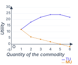
Drawn by us to help you understand the concept clearly, and verified to make sure it's accurate. For exams, practice from your textbook's own diagram.
Figure 2.1 is a standard two-curve graph that every Class 12 student must be able to read and interpret. On the horizontal axis (x-axis) you have Quantity of the commodity, labelled from 1 to 6 units. On the vertical axis (y-axis) you have Utility, ranging from -5 to 30. Two curves are plotted on the same set of axes.
The Total Utility (TU) curve starts at the origin (0,0) and rises steeply at first. At 1 unit, TU is 12; at 2 units, it is 18; at 3 units, 22; and at 4 units, 24. Notice that the increase from one unit to the next is getting smaller — this is the "diminishing rate" mentioned in the caption. The TU curve reaches its peak of 24 at the 4th unit and stays at 24 for the 5th unit (so the curve is flat between units 4 and 5). After the 5th unit, TU falls to 22 at the 6th unit, so the curve slopes downward.
The Marginal Utility (MU) curve is a separate line that falls steadily. At 1 unit, MU is 12; at 2 units, it drops to 6; at 3 units, to 4; at 4 units, to 2; at 5 units, it hits 0; and at 6 units, it becomes negative at -2. This line crosses the horizontal axis (the zero line) exactly at the 5th unit. The MU curve is always below the TU curve (since MU is the slope of TU, and TU is rising at a diminishing rate, then flat, then falling).
What the two curves together teach
The TU curve rises as long as MU is positive. When MU becomes zero (at the 5th unit), TU stops rising and is at its maximum. When MU turns negative (at the 6th unit), TU starts to fall. This is the core relationship: MU is the slope of TU. The law of diminishing marginal utility is visible in the steady downward slope of the MU curve — each additional unit adds less to total satisfaction than the previous one. …
Deriving the Demand Curve for a Single Commodity
Cardinal utility analysis gives us a direct way to understand why demand curves slope downward. But first, we need to be clear about what demand and the demand curve mean.
Demand for a commodity is the quantity a consumer is willing and able to buy, given the prices of goods and the consumer's income. It is not just a wish — the consumer must have the purchasing power to back it up. Demand for a good depends on:
- the price of itself,
- the prices of other goods (substitutes and complements),
- the consumer's income,
- the consumer's tastes and preferences.
The demand curve is a graph that shows the different quantities of a commodity a consumer is willing to buy at different prices of that same commodity, while holding constant everything else — prices of other goods, income, and tastes.
Figure 2.2 in the textbook shows a hypothetical demand curve for an individual consumer for commodity . The horizontal axis measures quantity, the vertical axis measures price. The curve slopes downward from left to right. At lower prices, the consumer buys more of ; at higher prices, she buys less. This negative relationship between price and quantity demanded is called the law of demand.
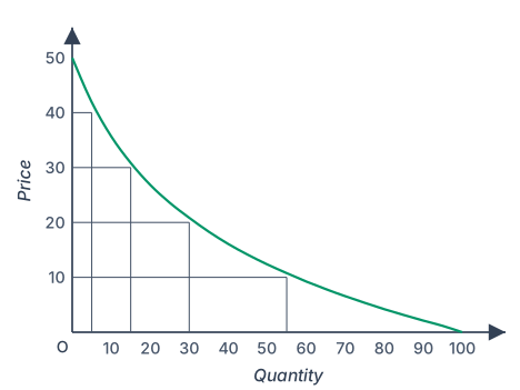
Drawn by us to help you understand the concept clearly, and verified to make sure it's accurate. For exams, practice from your textbook's own diagram.
Figure 2.2 is a simple two-axis graph. The vertical axis is labelled Price and runs from 10 to 50 (in rupees). The horizontal axis is labelled Quantity and runs from 10 to 100 (units of commodity x). A single, smooth curve is drawn sloping downwards from left to right. The curve is convex to the origin — meaning it is steep near the top-left (where price is high and quantity is low) and gradually flattens out as it moves toward the bottom-right (where price is low and quantity is high). Four thin reference rectangles are drawn under the curve, marking the price-quantity pairs the curve passes through: at a price of 40 the quantity demanded is 5, at 30 it is 15, at 20 it is 30, and at 10 it is 55. Each rectangle steps from the price axis across to the curve and down to the quantity axis, tying the curve to the textbook's own example of the individual's demand for commodity x.
What this figure teaches is the Law of Demand as derived from the Law of Diminishing Marginal Utility. The downward slope visually captures the negative relationship between price and quantity demanded: as price falls, the consumer is willing to buy more of commodity x; as price rises, she buys less. The convex shape (steep at first, then flattening) is not accidental — it reflects the underlying logic of diminishing marginal utility.
Here is the reasoning the figure embodies. According to the cardinal utility approach, each additional unit of a commodity gives less marginal utility than the previous one. A consumer will only pay for a unit what that unit is worth to her in terms of utility. So, for the first few units, marginal utility is high, and she is willing to pay a high price. But as she consumes more, marginal utility falls, and she will only buy additional units if the price drops correspondingly. This is why the demand curve is steep at low quantities (high price, high marginal utility) and flattens at high quantities (low price, low marginal utility). The curve is convex to the origin because the rate at which marginal utility falls is not constant — it diminishes quickly at first and then more slowly, which translates into a demand curve that is steep initially and then becomes flatter. …
When drawing a demand curve, remember the ceteris paribus condition — "other things being equal." The curve only shows the effect of the good's own price on quantity demanded. If income or the price of a substitute changes, the entire curve shifts. …