Economics · Ch 2 — Theory of Consumer Behaviour

Deriving a Demand Curve from Indifference Curves and Budget Constraints

2.4.2

Deriving a Demand Curve from Indifference Curves and Budget Constraints

The demand curve for a good shows how much of it a consumer wants to buy at different prices. The textbook derives this curve step by step using the consumer's optimisation problem — the same indifference-curve and budget-line framework we have been using.

The Setup: Two Goods, Fixed Income

Consider a consumer who buys two goods: bananas ( $X_1$ ) and mangoes ( $X_2$ ). Her income is $M$ , and the market prices are $P_1$ for bananas and $P_2$ for mangoes. Initially, both prices and income are given.

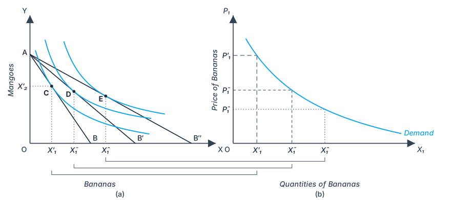
In panel (a) of Figure 2.14, the consumer reaches her utility-maximising equilibrium at point C. At this point, she buys $X_1'$ units of bananas and $X_2'$ units of mangoes. The budget line is tangent to the highest attainable indifference curve at C.

Now, in panel (b) of the same figure, we plot the price of bananas ( $P_1$ ) on the vertical axis against the quantity of bananas demanded ( $X_1$ ) on the horizontal axis. The first point on the demand curve for bananas is therefore $(X_1', P_1')$ — the price-quantity combination at the initial equilibrium.

A Drop in the Price of Bananas

Suppose the price of bananas falls from $P_1'$ to $P_1$ , while the price of mangoes ( $P_2'$ ) and the consumer's income ( $M$ ) remain unchanged. What happens?

The budget set expands — the budget line rotates outward, pivoting on the mangoes-intercept (since only the price of bananas changed). The consumer can now afford more of both goods. She re-optimises and reaches a new equilibrium at point D, which lies on a higher indifference curve. At D, she buys more bananas: $X_1 > X_1'$ .

In panel (b), we plot this new price $P_1$ against the new quantity $X_1$ , giving us the second point on the demand curve for bananas.

A Further Price Drop

The textbook then drops the price of bananas even further, to $\hat{P}_1$ . Again, the budget line rotates outward, and the consumer's new equilibrium is at a point where she buys $\hat{X}_1$ bananas — even more than before. Plotting $\hat{P}_1$ against $\hat{X}_1$ gives the third point on the demand curve.

Connecting these points yields a downward-sloping demand curve for bananas. The logic is clear: as the price of a good falls, a utility-maximising consumer buys more of it.

Figure 2.14Deriving a demand curve from indifference curves and budget constraints

Fig. 2.14 — Deriving a demand curve from indifference curves and budget constraints

Drawn by us to help you understand the concept clearly, and verified to make sure it's accurate. For exams, practice from your textbook's own diagram.

Figure 2.14 has two panels, arranged side by side. Panel (a) is the standard indifference-curve diagram: the vertical axis measures mangoes ( $X_2$ ), the horizontal axis measures bananas ( $X_1$ ). The consumer’s income $M$ and the price of mangoes $P_2$ are held fixed throughout. What changes is the price of bananas.

Three budget lines are drawn, all sharing the same vertical intercept on the mango axis — that intercept is $M/P_2$ , the maximum mangoes the consumer can buy if she spends all her income on mangoes. Because the price of bananas falls, each successive budget line pivots outward from this fixed point, becoming flatter. The highest budget line (the flattest one) corresponds to the lowest price of bananas; the steepest budget line corresponds to the highest price.

On each budget line, the consumer’s optimal bundle is the point where the budget line is tangent to an indifference curve. These tangency points are labelled C, D, and E, moving from the steepest budget line to the flattest. At point C, the quantity of bananas is $X'_1$ ; at point D, it is $\bar{X}_1$ (larger than $X'_1$ ); at point E, it is $\hat{X}_1$ (larger still). The indifference curves are successively higher — the consumer reaches a higher level of satisfaction as bananas become cheaper.

Panel (b) is a separate graph with the price of bananas on the vertical axis ( $P_1$ ) and the quantity of bananas on the horizontal axis ( $X_1$ ). Three points are plotted here. The first point corresponds to the highest price $P'_1$ and the smallest quantity $X'_1$ from point C in panel (a). The second point uses the middle price $\bar{P}_1$ and the middle quantity $\bar{X}_1$ from point D. The third point uses the lowest price $\hat{P}_1$ and the largest quantity $\hat{X}_1$ from point E. A single smooth, convex downward-sloping curve — labelled Demand — passes through these three points and extends beyond them at both ends: the individual demand curve for bananas. …

Note

This derivation assumes that only the price of the good in question changes. All other factors — income, prices of other goods, tastes — are held constant. This is the ceteris paribus condition that underlies the law of demand.

Why Does Demand Slope Downward? Two Effects

The negative slope of the demand curve can be explained by two distinct effects that occur when the price of a good changes.

Substitution effect. When bananas become cheaper relative to mangoes, the consumer substitutes bananas for mangoes. She rearranges her consumption basket to get the same level of satisfaction at a lower cost — or, more precisely, she moves along an indifference curve to a point where the marginal rate of substitution equals the new price ratio. This substitution effect always works to increase the demand for the good whose price has fallen.

Income effect. A drop in the price of bananas increases the consumer's real purchasing power. With the same money income, she can now afford more of both goods. This increase in real income leads to an increase in demand for bananas (and, typically, for mangoes as well). The income effect reinforces the substitution effect for a normal good, causing a further increase in the quantity demanded.

Together, these two effects ensure that a fall in price leads to a rise in quantity demanded — the demand curve slopes downward.

Watch out

The income effect can work in the opposite direction for an inferior good (a good whose demand falls when income rises). In that case, the income effect partially offsets the substitution effect. But for most goods — normal goods — both effects work in the same direction, and the demand curve is unambiguously downward sloping.

The Law of Demand

The textbook states the law of demand formally:

Law of Demand: Other things being equal, there is a negative relation between the demand for a commodity and its price. In other words, when the price of a commodity increases, demand for it falls; when the price decreases, demand for it rises — provided all other factors remain the same.

This law is the foundation of the demand curve we have just derived.

Linear Demand Curve

The textbook introduces a specific functional form for the demand curve — the linear demand curve. It is written as:

d(p) = a - bp, \quad 0 \leq p \leq \frac{a}{b}

where: …

Figure 2.15Linear Demand Curve. The diagram depicts the linear demand curve given by equation 2.13.

Fig. 2.15 — Linear Demand Curve. The diagram depicts the linear demand curve given by equation 2.13.

Drawn by us to help you understand the concept clearly, and verified to make sure it's accurate. For exams, practice from your textbook's own diagram.

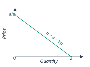
The figure shows a standard two-axis graph. The vertical axis is labelled Price and the horizontal axis is labelled Quantity. A single straight line slopes downward from left to right, crossing both axes. This line is the linear demand curve.

The point where the demand curve meets the vertical (Price) axis is labelled $a/b$ . This is the vertical intercept — the price at which quantity demanded becomes zero. The point where the demand curve meets the horizontal (Quantity) axis is labelled $a$ . This is the horizontal intercept — the quantity demanded when the price is zero.

The equation of this line is written on the diagram as $q = a - bp$ , where $q$ stands for quantity demanded and $p$ stands for price. The parameters $a$ and $b$ are positive constants. The slope of the line is $-b$ , which is negative — confirming the inverse relationship between price and quantity demanded. …

Start your 14-day free trial to unlock the full solution →

← Previous · 2.4.1Demand Curve and the Law of Demand Next · 2.4.3 →Normal and Inferior Goods