Mathematics · Ch 6 — Limits and Derivatives

Limits of Trigonometric Functions

6.4

Limits of Trigonometric Functions

Before we can evaluate limits involving trigonometric functions, we need two general theorems about limits of functions. These theorems are not about trigonometry themselves — they are tools that work for any functions, and they become essential when we handle trigonometric limits.

Theorem 3: Inequality Preservation Under Limits

If $f$ and $g$ are two real-valued functions defined on the same domain, and $f(x) \leq g(x)$ for every $x$ in that domain, then for any real number $a$ :

If both $\lim_{x \to a} f(x)$ and $\lim_{x \to a} g(x)$ exist, then

\lim_{x \to a} f(x) \leq \lim_{x \to a} g(x)

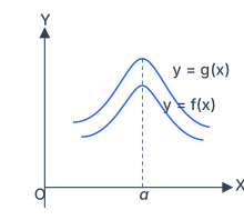
This is intuitive: if one function never exceeds another, its limit cannot exceed the other's limit either. The textbook illustrates this with Fig 12.8, where the graph of $f$ stays below the graph of $g$ near $x = a$ , and the limits reflect that ordering.

Watch out

This theorem only applies when both limits exist. If either limit does not exist, the inequality between the functions does not guarantee anything about the limits.

Theorem 4: The Sandwich Theorem (Squeeze Theorem)

Let $f$ , $g$ , and $h$ be real functions such that

f(x) \leq g(x) \leq h(x)

for all $x$ in their common domain of definition. For some real number $a$ , if

\lim_{x \to a} f(x) = l = \lim_{x \to a} h(x)

then

\lim_{x \to a} g(x) = l

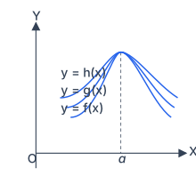
Think of it this way: if $g$ is "sandwiched" between $f$ and $h$ , and both the bottom and top functions approach the same number $l$ , then $g$ has no choice but to also approach $l$ . The textbook shows this in Fig 12.9 — the middle function is trapped between the other two near $x = a$ .

Tip

The Sandwich Theorem is your primary weapon for proving $\lim_{x \to 0} \frac{\sin x}{x} = 1$ . You find functions that bound $\frac{\sin x}{x}$ from above and below, both approaching 1, and the theorem does the rest.

The Fundamental Inequality: $\cos x < \frac{\sin x}{x} < 1$ for $0 < x < \frac{\pi}{2}$

The textbook gives a geometric proof of this inequality, which is the foundation for the two standard trigonometric limits. Here is the complete reasoning.

›Proof

Geometric proof of $\cos x < \frac{\sin x}{x} < 1$ for $0 < x < \frac{\pi}{2}$

Since $\sin(-x) = -\sin x$ and $\cos(-x) = \cos x$ , the inequality for negative $x$ follows from the positive case. So we only need to prove it for $0 < x < \frac{\pi}{2}$ .

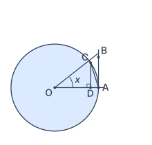
Consider a unit circle (radius $= 1$ ) with centre $O$ . Let $\angle AOC = x$ radians, where $0 < x < \frac{\pi}{2}$ . Draw perpendiculars $BA$ and $CD$ to $OA$ . Join $AC$ .

Now compare three areas:

Area of $\triangle OAC = \frac{1}{2} \cdot OA \cdot CD$
Area of sector $OAC = \frac{x}{2\pi} \cdot \pi \cdot (OA)^2 = \frac{1}{2} \cdot x \cdot (OA)^2$
Area of $\triangle OAB = \frac{1}{2} \cdot OA \cdot AB$

From the geometry, these areas satisfy:

$\text{Area}(\triangle OAC) < \text{Area}(\text{sector } OAC) < \text{Area}(\triangle OAB)$

Substituting the expressions:

$\frac{1}{2} \cdot OA \cdot CD < \frac{1}{2} \cdot x \cdot (OA)^2 < \frac{1}{2} \cdot OA \cdot AB$

Cancelling $\frac{1}{2} \cdot OA$ (which is positive):

$CD < x \cdot OA < AB$

From $\triangle OCD$ , $\sin x = \frac{CD}{OC} = \frac{CD}{OA}$ (since $OC = OA = 1$ ), so $CD = OA \sin x$ .

From $\triangle OAB$ , $\tan x = \frac{AB}{OA}$ , so $AB = OA \tan x$ .

Substituting:

$OA \sin x < OA \cdot x < OA \tan x$

Since $OA > 0$ , divide through by $OA$ :

$\sin x < x < \tan x$

Now $0 < x < \frac{\pi}{2}$ means $\sin x > 0$ . Divide the entire inequality by $\sin x$ :

$1 < \frac{x}{\sin x} < \frac{1}{\cos x}$

Taking reciprocals (which reverses the inequalities because all terms are positive):

$\cos x < \frac{\sin x}{x} < 1$

This completes the proof.

Theorem 5: The Two Fundamental Trigonometric Limits

The textbook presents these as the central results of the section.

(i) $\displaystyle \lim_{x \to 0} \frac{\sin x}{x} = 1$

›Proof

From the inequality we just proved:

$\cos x < \frac{\sin x}{x} < 1 \quad \text{for } 0 < |x| < \frac{\pi}{2}$

The function $\frac{\sin x}{x}$ is sandwiched between $\cos x$ and the constant function $1$ .

We know $\lim_{x \to 0} \cos x = 1$ (by direct substitution, since cosine is continuous).

So both the lower bound ( $\cos x$ ) and the upper bound ( $1$ ) approach $1$ as $x \to 0$ .

By the Sandwich Theorem:

$\lim_{x \to 0} \frac{\sin x}{x} = 1$

Important

This limit is not obtained by direct substitution. If you plug $x = 0$ into $\frac{\sin x}{x}$ , you get $\frac{0}{0}$ , which is indeterminate. The Sandwich Theorem is what saves us.

(ii) $\displaystyle \lim_{x \to 0} \frac{1 - \cos x}{x} = 0$

›Proof

Use the trigonometric identity $1 - \cos x = 2 \sin^2 \frac{x}{2}$ .

$\lim_{x \to 0} \frac{1 - \cos x}{x} = \lim_{x \to 0} \frac{2 \sin^2 \frac{x}{2}}{x}$

Rewrite by multiplying numerator and denominator strategically:

$= \lim_{x \to 0} \frac{2 \sin \frac{x}{2} \cdot \sin \frac{x}{2}}{x}$

$= \lim_{x \to 0} \left( \frac{\sin \frac{x}{2}}{\frac{x}{2}} \cdot \sin \frac{x}{2} \right)$

As $x \to 0$ , we have $\frac{x}{2} \to 0$ . So let $y = \frac{x}{2}$ . Then:

$= \lim_{y \to 0} \left( \frac{\sin y}{y} \cdot \sin y \right)$

$= \left( \lim_{y \to 0} \frac{\sin y}{y} \right) \cdot \left( \lim_{y \to 0} \sin y \right)$

$= 1 \cdot 0 = 0$

Note

The step where we replace $x \to 0$ with $\frac{x}{2} \to 0$ is valid because if $x$ approaches 0, then $\frac{x}{2}$ also approaches 0. This substitution trick — setting $y = \frac{x}{2}$ — is extremely common in limit problems.

--- …

Theorem 3

Theorem 5: Two Important Trigonometric Limits

The theorem states two fundamental limits that form the backbone of evaluating limits involving trigonometric functions:

\lim_{x \to 0} \frac{\sin x}{x} = 1

Both limits hold when $x$ is measured in radians. The first limit is the more critical one — it tells us that near zero, $\sin x$ behaves almost exactly like $x$ itself. The second limit follows directly from the first using a trigonometric identity.

Watch out

A common mistake is to think $\lim_{x \to 0} \frac{\sin x}{x} = 0$ because $\sin 0 = 0$ . But the denominator also goes to zero, so the limit is an indeterminate form $\frac{0}{0}$ — it requires careful analysis, not direct substitution.

Proof of $\displaystyle \lim_{x \to 0} \frac{\sin x}{x} = 1$

The proof uses the Sandwich Theorem (Theorem 4 from the textbook) together with a geometric inequality.

›Proof

Step 1: Establish the inequality for $0 < x < \frac{\pi}{2}$

Consider a unit circle centred at $O$ . Let $\angle AOC = x$ radians, with $0 < x < \frac{\pi}{2}$ . Draw perpendiculars $BA$ and $CD$ to $OA$ , and join $AC$ .

From the geometry, we have:

$\text{Area of } \triangle OAC < \text{Area of sector } OAC < \text{Area of } \triangle OAB$

Computing each area:

$\frac{1}{2} \cdot OA \cdot CD < \frac{1}{2\pi} \cdot \pi \cdot (OA)^2 \cdot x < \frac{1}{2} \cdot OA \cdot AB$

Since $OA = 1$ (unit circle), this simplifies to:

$CD < x < AB$

Step 2: Express $CD$ and $AB$ in trigonometric terms

From $\triangle OCD$ : $\sin x = \frac{CD}{OC} = \frac{CD}{1}$ , so $CD = \sin x$ .

From $\triangle OAB$ : $\tan x = \frac{AB}{OA} = \frac{AB}{1}$ , so $AB = \tan x$ .

Substituting into the inequality:

$\sin x < x < \tan x$

Step 3: Manipulate to get the sandwich

Since $0 < x < \frac{\pi}{2}$ , $\sin x > 0$ . Divide the entire inequality by $\sin x$ :

$1 < \frac{x}{\sin x} < \frac{1}{\cos x}$

Taking reciprocals reverses the inequalities (all terms are positive):

$\cos x < \frac{\sin x}{x} < 1$

Step 4: Apply the Sandwich Theorem

We know $\displaystyle \lim_{x \to 0} \cos x = 1$ and the constant function $1$ also has limit $1$ . The function $\frac{\sin x}{x}$ is sandwiched between $\cos x$ and $1$ for $0 < x < \frac{\pi}{2}$ .

Since $\sin(-x) = -\sin x$ and $\cos(-x) = \cos x$ , the inequality $\cos x < \frac{\sin x}{x} < 1$ also holds for $-\frac{\pi}{2} < x < 0$ (check: $\frac{\sin(-x)}{-x} = \frac{-\sin x}{-x} = \frac{\sin x}{x}$ , and $\cos(-x) = \cos x$ ).

Therefore, by the Sandwich Theorem:

$\lim_{x \to 0} \frac{\sin x}{x} = 1$

Proof of $\displaystyle \lim_{x \to 0} \frac{1 - \cos x}{x} = 0$

This proof uses the first limit together with a standard trigonometric identity.

›Proof

Step 1: Use the half-angle identity

Recall: $1 - \cos x = 2 \sin^2 \frac{x}{2}$ .

Therefore:

$\frac{1 - \cos x}{x} = \frac{2 \sin^2 \frac{x}{2}}{x} = \frac{2 \sin \frac{x}{2} \cdot \sin \frac{x}{2}}{x}$

Step 2: Rewrite to use the known limit

Multiply numerator and denominator to create the form $\frac{\sin \theta}{\theta}$ :

$\frac{1 - \cos x}{x} = \frac{\sin \frac{x}{2}}{\frac{x}{2}} \cdot \sin \frac{x}{2}$

Step 3: Take the limit

As $x \to 0$ , we have $\frac{x}{2} \to 0$ . Using the first limit:

$\lim_{x \to 0} \frac{\sin \frac{x}{2}}{\frac{x}{2}} = 1$

And $\displaystyle \lim_{x \to 0} \sin \frac{x}{2} = 0$ .

Hence:

$\lim_{x \to 0} \frac{1 - \cos x}{x} = 1 \cdot 0 = 0$ …

Theorem 4

Theorem 5: Two Important Trigonometric Limits

The theorem states two fundamental limits that form the backbone of evaluating limits involving trigonometric functions:

\lim_{x \to 0} \frac{\sin x}{x} = 1

Watch out

Proof of $\displaystyle \lim_{x \to 0} \frac{\sin x}{x} = 1$

The proof uses the Sandwich Theorem (Theorem 4 from the textbook) together with a geometric inequality.

›Proof

Step 1: Establish the inequality for $0 < x < \frac{\pi}{2}$

Consider a unit circle centred at $O$ . Let $\angle AOC = x$ radians, with $0 < x < \frac{\pi}{2}$ . Draw perpendiculars $BA$ and $CD$ to $OA$ , and join $AC$ .

From the geometry, we have:

$\text{Area of } \triangle OAC < \text{Area of sector } OAC < \text{Area of } \triangle OAB$

Computing each area:

$\frac{1}{2} \cdot OA \cdot CD < \frac{1}{2\pi} \cdot \pi \cdot (OA)^2 \cdot x < \frac{1}{2} \cdot OA \cdot AB$

Since $OA = 1$ (unit circle), this simplifies to:

$CD < x < AB$

Step 2: Express $CD$ and $AB$ in trigonometric terms

From $\triangle OCD$ : $\sin x = \frac{CD}{OC} = \frac{CD}{1}$ , so $CD = \sin x$ .

From $\triangle OAB$ : $\tan x = \frac{AB}{OA} = \frac{AB}{1}$ , so $AB = \tan x$ .

Substituting into the inequality:

$\sin x < x < \tan x$

Step 3: Manipulate to get the sandwich

Since $0 < x < \frac{\pi}{2}$ , $\sin x > 0$ . Divide the entire inequality by $\sin x$ :

$1 < \frac{x}{\sin x} < \frac{1}{\cos x}$

Taking reciprocals reverses the inequalities (all terms are positive):

$\cos x < \frac{\sin x}{x} < 1$

Step 4: Apply the Sandwich Theorem

Therefore, by the Sandwich Theorem:

$\lim_{x \to 0} \frac{\sin x}{x} = 1$

Proof of $\displaystyle \lim_{x \to 0} \frac{1 - \cos x}{x} = 0$

This proof uses the first limit together with a standard trigonometric identity.

›Proof

Step 1: Use the half-angle identity

Recall: $1 - \cos x = 2 \sin^2 \frac{x}{2}$ .

Therefore:

$\frac{1 - \cos x}{x} = \frac{2 \sin^2 \frac{x}{2}}{x} = \frac{2 \sin \frac{x}{2} \cdot \sin \frac{x}{2}}{x}$

Step 2: Rewrite to use the known limit

Multiply numerator and denominator to create the form $\frac{\sin \theta}{\theta}$ :

$\frac{1 - \cos x}{x} = \frac{\sin \frac{x}{2}}{\frac{x}{2}} \cdot \sin \frac{x}{2}$

Step 3: Take the limit

As $x \to 0$ , we have $\frac{x}{2} \to 0$ . Using the first limit:

$\lim_{x \to 0} \frac{\sin \frac{x}{2}}{\frac{x}{2}} = 1$

And $\displaystyle \lim_{x \to 0} \sin \frac{x}{2} = 0$ .

Hence:

$\lim_{x \to 0} \frac{1 - \cos x}{x} = 1 \cdot 0 = 0$ …

Theorem 5

Theorem 5: Two Important Trigonometric Limits

The theorem states two fundamental limits that form the backbone of evaluating limits involving trigonometric functions:

\lim_{x \to 0} \frac{\sin x}{x} = 1

Watch out

Proof of $\displaystyle \lim_{x \to 0} \frac{\sin x}{x} = 1$

The proof uses the Sandwich Theorem (Theorem 4 from the textbook) together with a geometric inequality.

›Proof

Step 1: Establish the inequality for $0 < x < \frac{\pi}{2}$

Consider a unit circle centred at $O$ . Let $\angle AOC = x$ radians, with $0 < x < \frac{\pi}{2}$ . Draw perpendiculars $BA$ and $CD$ to $OA$ , and join $AC$ .

From the geometry, we have:

$\text{Area of } \triangle OAC < \text{Area of sector } OAC < \text{Area of } \triangle OAB$

Computing each area:

$\frac{1}{2} \cdot OA \cdot CD < \frac{1}{2\pi} \cdot \pi \cdot (OA)^2 \cdot x < \frac{1}{2} \cdot OA \cdot AB$

Since $OA = 1$ (unit circle), this simplifies to:

$CD < x < AB$

Step 2: Express $CD$ and $AB$ in trigonometric terms

From $\triangle OCD$ : $\sin x = \frac{CD}{OC} = \frac{CD}{1}$ , so $CD = \sin x$ .

From $\triangle OAB$ : $\tan x = \frac{AB}{OA} = \frac{AB}{1}$ , so $AB = \tan x$ .

Substituting into the inequality:

$\sin x < x < \tan x$

Step 3: Manipulate to get the sandwich

Since $0 < x < \frac{\pi}{2}$ , $\sin x > 0$ . Divide the entire inequality by $\sin x$ :

$1 < \frac{x}{\sin x} < \frac{1}{\cos x}$

Taking reciprocals reverses the inequalities (all terms are positive):

$\cos x < \frac{\sin x}{x} < 1$

Step 4: Apply the Sandwich Theorem

Therefore, by the Sandwich Theorem:

$\lim_{x \to 0} \frac{\sin x}{x} = 1$

Proof of $\displaystyle \lim_{x \to 0} \frac{1 - \cos x}{x} = 0$

This proof uses the first limit together with a standard trigonometric identity.

›Proof

Step 1: Use the half-angle identity

Recall: $1 - \cos x = 2 \sin^2 \frac{x}{2}$ .

Therefore:

$\frac{1 - \cos x}{x} = \frac{2 \sin^2 \frac{x}{2}}{x} = \frac{2 \sin \frac{x}{2} \cdot \sin \frac{x}{2}}{x}$

Step 2: Rewrite to use the known limit

Multiply numerator and denominator to create the form $\frac{\sin \theta}{\theta}$ :

$\frac{1 - \cos x}{x} = \frac{\sin \frac{x}{2}}{\frac{x}{2}} \cdot \sin \frac{x}{2}$

Step 3: Take the limit

As $x \to 0$ , we have $\frac{x}{2} \to 0$ . Using the first limit:

$\lim_{x \to 0} \frac{\sin \frac{x}{2}}{\frac{x}{2}} = 1$

And $\displaystyle \lim_{x \to 0} \sin \frac{x}{2} = 0$ .

Hence:

$\lim_{x \to 0} \frac{1 - \cos x}{x} = 1 \cdot 0 = 0$ …

Figure 12.8Two functions with f(x) ≤ g(x): comparing limits at x=a

Fig. 12.8 — Two functions with f(x) ≤ g(x): comparing limits at x=a

Drawn by us to help you understand the concept clearly, and verified to make sure it's accurate. For exams, practice from your textbook's own diagram.

Fig. 12.8 is a simple but powerful visual proof of Theorem 3: if one function never goes above another, the same ordering holds for their limits.

The figure shows the first quadrant of the $xy$ -plane, with axes labelled $X$ (horizontal) and $Y$ (vertical). Two smooth, bell-shaped curves are drawn in blue. The upper curve is labelled $y = g(x)$ ; the lower curve is labelled $y = f(x)$ . At every $x$ shown, the $g$ -curve lies strictly above the $f$ -curve — that is, $f(x) \le g(x)$ for all $x$ in the domain. A dashed vertical line is drawn at $x = a$ , cutting through both curves. The curves peak near $x = a$ , so the values $f(a)$ and $g(a)$ are close to their respective maxima, but the key point is that the entire $g$ -curve sits above the $f$ -curve.

What does this teach? If $f(x) \le g(x)$ everywhere, then as $x$ approaches $a$ , the limit of $f$ cannot exceed the limit of $g$ . The dashed line at $x = a$ helps you visualise the limiting values: imagine the $y$ -coordinates where the curves meet that line. Even if the functions are not defined exactly at $x = a$ , the limits (the $y$ -values the curves approach) must obey the same inequality. The figure makes this obvious — the upper curve's limit is higher, the lower curve's limit is lower, and they cannot cross.

The central result illustrated is Theorem 3:

\text{If } f(x) \le g(x) \text{ for all } x \text{ in the domain, and } \lim_{x \to a} f(x) \text{ and } \lim_{x \to a} g(x) \text{ exist, then } \lim_{x \to a} f(x) \le \lim_{x \to a} g(x).

This theorem is the stepping stone to the far more powerful Sandwich Theorem (Theorem 4), shown in the next figure (Fig. 12.9). There, a third function $h(x)$ is added above $g(x)$ , so $f(x) \le g(x) \le h(x)$ . If the outer two functions both approach the same limit $l$ , then $g(x)$ is forced to approach $l$ as well — it is "sandwiched" between them. The inequality $\cos x < \frac{\sin x}{x} < 1$ for $0 < x < \frac{\pi}{2}$ is the classic example, and the Sandwich Theorem then gives $\lim_{x \to 0} \frac{\sin x}{x} = 1$ . …

Figure 12.9Sandwich Theorem: f ≤ g ≤ h squeezing g to the common limit at x=a

Fig. 12.9 — Sandwich Theorem: f ≤ g ≤ h squeezing g to the common limit at x=a

Drawn by us to help you understand the concept clearly, and verified to make sure it's accurate. For exams, practice from your textbook's own diagram.

Fig 12.9 is the visual statement of the Sandwich Theorem (also called the Squeeze Theorem). The axes are the standard first-quadrant pair: the horizontal axis is labelled $X$ , the vertical axis $Y$ , and the origin is $O$ . Three curves are drawn in blue, each representing a different function of $x$ .

The top curve is $y = h(x)$ , the middle curve is $y = g(x)$ , and the bottom curve is $y = f(x)$ . A dashed vertical line is drawn at $x = a$ . The critical visual fact is that all three curves converge to a single point directly above $x = a$ — that is, they meet at the same height on the $Y$ -axis. After passing that point, the curves fan out again: $h$ rises above, $f$ drops below, and $g$ stays sandwiched between them.

The physical idea is straightforward. If $f(x)$ and $h(x)$ are two functions that "squeeze" $g(x)$ from below and above for all $x$ near $a$ (except possibly at $a$ itself), and if both $f$ and $h$ approach the same number $l$ as $x$ approaches $a$ , then $g$ is forced to approach that same number $l$ . The figure shows this squeezing action: the three curves are distinct away from $x = a$ , but they are pinched together at the limit point. The dashed vertical line at $x = a$ marks the location where the limit is being taken — note that the curves may or may not actually pass through that point; the theorem only cares about behaviour near $a$ , not at $a$ .

The textbook uses this figure to introduce Theorem 4 (Sandwich Theorem):

\text{If } f(x) \le g(x) \le h(x) \text{ for all } x \text{ (in a common domain), and } \lim_{x \to a} f(x) = l = \lim_{x \to a} h(x), \text{ then } \lim_{x \to a} g(x) = l.

Here $f$ , $g$ , $h$ are real-valued functions, $a$ is a real number, and $l$ is the common limit. The figure directly illustrates this: $f$ (bottom curve) and $h$ (top curve) both approach the same height $l$ at $x = a$ , so the middle curve $g$ is "squeezed" to that same height.

The textbook then applies this theorem to prove the fundamental trigonometric limit:

\lim_{x \to 0} \frac{\sin x}{x} = 1.

The proof uses the inequality $\cos x < \frac{\sin x}{x} < 1$ for $0 < x < \frac{\pi}{2}$ , which is exactly a sandwich: $f(x) = \cos x$ , $g(x) = \frac{\sin x}{x}$ , $h(x) = 1$ . Since $\lim_{x \to 0} \cos x = 1$ and $\lim_{x \to 0} 1 = 1$ , the Sandwich Theorem forces $\lim_{x \to 0} \frac{\sin x}{x} = 1$ . The figure in the textbook (Fig 12.9) is the generic picture of this idea; the specific trigonometric inequality is then proved geometrically using a unit circle diagram (Fig 12.10). …

Figure 12.10Unit circle: area(△OAC) < area(sector OAC) < area(△OAB) for angle x

Fig. 12.10 — Unit circle: area(△OAC) < area(sector OAC) < area(△OAB) for angle x

Drawn by us to help you understand the concept clearly, and verified to make sure it's accurate. For exams, practice from your textbook's own diagram.

Fig 12.10 is a geometric construction inside a unit circle — a circle with centre O and radius 1. The radius OA is drawn horizontally to the right, ending at point A on the circumference. From the centre O, a second radius OC is drawn at an angle $x$ (measured anticlockwise from OA), so that the angle $\angle AOC = x$ radians. The figure is drawn for a small positive angle, $0 < x < \frac{\pi}{2}$ .

From point C, a perpendicular CD is dropped to OA, meeting OA at D. A right-angle mark is shown at D. The chord AC is drawn. At point A, a vertical line (the tangent to the circle at A) is drawn upward; it meets the extension of OC at point B. So AB is vertical, and OA is horizontal, making triangle OAB a right triangle with the right angle at A.

The figure contains three regions, all shaded in light blue: triangle OAC (bounded by OA, OC, and chord AC), sector OAC (the pie-slice of the circle between radii OA and OC), and triangle OAB (bounded by OA, OB, and the tangent segment AB). The key visual idea is that these three regions are nested inside each other — triangle OAC lies entirely inside the sector, which in turn lies entirely inside triangle OAB. Because area is a positive quantity, this gives the inequality chain:

\text{area}(\triangle OAC) \;<\; \text{area}(\text{sector } OAC) \;<\; \text{area}(\triangle OAB)

Now we express each area in terms of $x$ and the radius (which is 1). For triangle OAC, base OA = 1 and height CD = $\sin x$ (since in right triangle OCD, $\sin x = \frac{CD}{OC} = \frac{CD}{1}$ ). So its area is $\frac12 \cdot 1 \cdot \sin x = \frac12 \sin x$ .

For sector OAC, the area of a sector of angle $x$ in a unit circle is $\frac12 x$ (since full circle area $\pi \cdot 1^2$ corresponds to angle $2\pi$ , so area $= \frac{x}{2\pi} \cdot \pi = \frac{x}{2}$ ). So sector area $= \frac12 x$ .

For triangle OAB, base OA = 1 and height AB = $\tan x$ (since in right triangle OAB, $\tan x = \frac{AB}{OA} = \frac{AB}{1}$ ). Its area is $\frac12 \cdot 1 \cdot \tan x = \frac12 \tan x$ .

Substituting these into the inequality and multiplying through by 2 gives:

\sin x \;<\; x \;<\; \tan x \qquad \text{for } 0 < x < \frac{\pi}{2}

This is the fundamental inequality the figure is designed to prove. From it, by dividing by $\sin x$ (positive in this interval) and taking reciprocals, the textbook obtains the sandwich inequality:

\cos x \;<\; \frac{\sin x}{x} \;<\; 1 \qquad \text{for } 0 < x < \frac{\pi}{2}

This inequality is the heart of the proof that $\displaystyle \lim_{x \to 0} \frac{\sin x}{x} = 1$ , using the Sandwich Theorem (Theorem 4). As $x \to 0$ , $\cos x \to 1$ , so the function $\frac{\sin x}{x}$ , trapped between 1 and a function approaching 1, must also approach 1.

Note

The figure uses a unit circle (radius = 1) so that lengths like $\sin x$ and $\tan x$ appear directly as segment lengths — CD and AB respectively — without scaling factors. This is why the area expressions simplify so cleanly. …

Start your 14-day free trial to unlock the full solution →

← Previous · 6.3.2Example 3 — Evaluate: (i) limx→ 1dfracx¹⁵ - 1x¹⁰ - 1 (ii) limx→ 0dfrac√(1 + x) - 1…Next · 6.4 →Example 4 — Evaluate: (i) limx→ 0(sin 4x)/(sin 2x) (ii) limx→ 0(tan x)/(x)

Limits of Trigonometric Functions