Mathematics · Ch 1 — Relations and Functions
Some Functions and Their Graphs
Some Functions and Their Graphs
Some Functions and Their Graphs
The Identity Function
The simplest function you will encounter is the identity function. Let be the set of real numbers. Define by
For every input, the output is exactly the same number. The domain is (all real numbers) and the range is also .
The graph of is a straight line that passes through the origin, making a angle with both axes. Every point on this line has coordinates for some real .
The identity function is the simplest example of a one-to-one and onto function. It maps every real number to itself — nothing is lost or gained.
The Constant Function
Define by
where is a fixed real constant. The domain is , but the range is the single-element set .
The graph is a horizontal straight line parallel to the -axis, passing through the point . For instance, if for every , the graph is the line .
A constant function is not one-to-one (many inputs give the same output), but it is a perfectly valid function. Do not confuse "constant" with "identity" — they behave very differently.
Polynomial Functions
A function is called a polynomial function if for each ,
where is a non-negative integer and .
The highest power is the degree of the polynomial. The coefficients are real numbers.
Examples of polynomial functions:
- (degree 3)
- (degree 4)
Non-example: is not a polynomial function. Why? Because the term can be rewritten as , and the exponent is not a non-negative integer. Polynomials require non-negative integer exponents only.
Example:
Define by . Complete the table:
Domain: — all real numbers.
Range: — all non-negative real numbers .
The graph is a parabola opening upward, symmetric about the -axis, with its vertex at the origin .
Example:
Define by .
Some values: , , , , , , .
So .
The graph is a cubic curve that passes through the origin. Unlike , it is symmetric about the origin — for every point , there is a corresponding point . The curve increases steeply for positive and decreases steeply for negative .
For polynomial functions, the shape of the graph depends heavily on the degree. Even-degree polynomials (like ) have the same sign for large positive and large negative ; odd-degree polynomials (like ) have opposite signs.
Rational Functions
A rational function is a function of the form
where and are polynomial functions, and the function is defined only where .
The domain excludes any that makes the denominator zero.
Example:
Define by
Complete the table:
Domain: All real numbers except — written as or .
Range: Also all real numbers except — .
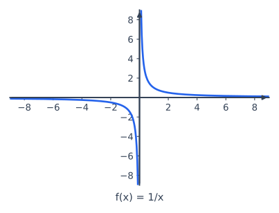
The graph is a rectangular hyperbola with two branches. One branch lies in the first quadrant (positive , positive ) and the other in the third quadrant (negative , negative ). The axes act as asymptotes — the curve approaches the -axis and -axis but never touches them.
For , as approaches from the positive side, becomes very large positive. As approaches from the negative side, becomes very large negative. This is why is excluded from the domain.
The Modulus Function
The modulus function (also called the absolute value function) is defined by with
The definition is piecewise:
For non-negative , the output equals itself. For negative , the output is the negative of — which makes it positive.
Domain: (all real numbers).
Range: (all non-negative real numbers).
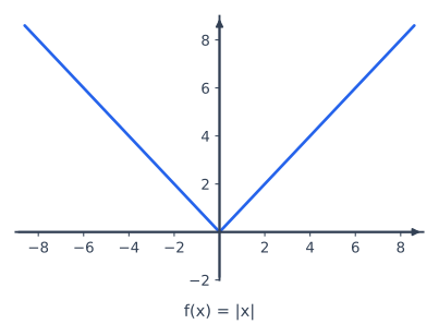
The graph consists of two rays meeting at the origin. For , it is the line (the identity function). For , it is the line , which has slope . The graph forms a V-shape with its vertex at .
The modulus function is always non-negative. It measures the distance of a number from zero on the number line, regardless of direction.
The Signum Function
The signum function (from Latin signum meaning "sign") is defined by with
This function tells you the sign of a real number: positive numbers give , negative numbers give , and zero gives .
Domain: (all real numbers).
Range: — just three possible values.
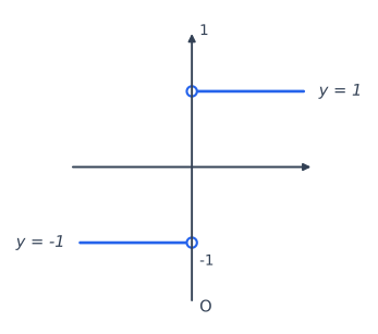
The graph has three distinct parts:
- For , a horizontal line at (open circle at )
- At , a single point at
- For , a horizontal line at (open circle at )
The signum function is not continuous at . There is a jump from to to at that point. The open circles on the graph indicate that the endpoints and are not attained at .
The Greatest Integer Function …
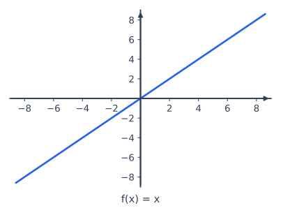
Drawn by us to help you understand the concept clearly, and verified to make sure it's accurate. For exams, practice from your textbook's own diagram.
The Graph of the Identity Function
The figure shows a standard Cartesian plane with both axes drawn as double-arrowed lines, extending from approximately −8 to 8 on each axis. Even-numbered tick marks are labelled along both axes. A single straight line, coloured indigo, runs through the origin at a 45° angle — it has slope exactly 1. The line has arrowheads at both ends, indicating it continues indefinitely in both directions.
Every point on this line satisfies the condition that its -coordinate equals its -coordinate. The line passes through , , , , , and so on. There are no breaks, no curves, no other lines — just this one diagonal.
What This Figure Teaches
The identity function is the simplest possible function that still does something: it takes each input and returns it unchanged. The graph makes this idea visually obvious. If you pick any on the horizontal axis, the corresponding on the vertical axis is exactly the same number. The line is the set of all points where the two coordinates are equal.
This is the baseline against which all other functions are compared. When you later study transformations — shifting, stretching, reflecting — the identity function is the starting point. A vertical shift upward by 2 units, for instance, turns into . A reflection across the -axis turns it into . Understanding the identity function's graph first makes those modifications easy to see.
The identity function is the only function whose graph is a straight line through the origin with slope 1. Its domain is (all real numbers) and its range is also .
The Key Formula
The central relationship the figure illustrates is:
Here:
- is the function name
- is the input variable (any real number)
- is the output, which equals the input
- denotes the set of all real numbers …
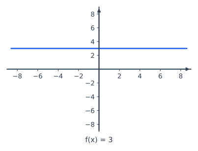
Drawn by us to help you understand the concept clearly, and verified to make sure it's accurate. For exams, practice from your textbook's own diagram.
The Graph of a Constant Function
Figure 2.9 shows the simplest possible non-trivial function: a constant function. The axes are the standard Cartesian frame — a horizontal -axis and a vertical -axis, meeting at the origin. Drawn across this plane is a single horizontal line at height , running parallel to the -axis. The line has arrowheads on both ends, indicating that it extends infinitely in both directions along the -axis.
The physical idea is straightforward: no matter what -value you choose, the output is always the same number. In this case, for every real . The graph is a horizontal line because the -coordinate never changes — it is constant. The line is perfectly flat, with zero slope.
Here is a fixed real number (the constant), and denotes the set of all real numbers. The domain of this function is (every real number is allowed as input), and the range is the single-element set — only one output value ever appears.
The line in the figure is at , so for this example. Every point on that line has coordinates of the form , where can be any real number. The line is parallel to the -axis because the -coordinate is fixed; it never rises or falls as changes.
A constant function is not the same as a function that is undefined or has no output. It produces exactly one output for every input — it just happens that the output is always identical. The graph is a horizontal line, not a single dot. …
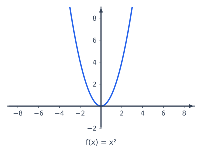
Drawn by us to help you understand the concept clearly, and verified to make sure it's accurate. For exams, practice from your textbook's own diagram.
The Graph of
Figure 2.10 shows the graph of the quadratic function , defined for all real numbers . The axes are drawn in the standard Cartesian plane: the horizontal -axis and vertical -axis intersect at the origin . The curve itself is an upward-opening parabola, coloured indigo in the textbook.
The parabola is symmetric about the -axis. This means the left half () is a mirror image of the right half (). The vertex — the lowest point on the curve — sits exactly at the origin. From there, the graph rises smoothly in both directions, becoming steeper as increases.
The table in Example 13 gives the key points plotted: , , , , , , , , . These points lie on the parabola and confirm its shape. The curve passes through every such point, forming a continuous, unbroken line.
The parabola never dips below the -axis because is never negative. Every output is either zero or positive.
What the Figure Teaches
The graph makes three ideas immediately visible.
First, domain and range. The domain of is all real numbers — you can square any real . The range, however, is only non-negative real numbers: . The graph stays on or above the -axis, showing that never takes a negative value.
Second, even symmetry. For any , . This is why the curve is symmetric about the -axis. Functions with this property are called even functions.
Third, the shape of a quadratic. The parabola is the simplest non-linear polynomial graph. Its U-shape, with a single minimum at the vertex, is the foundation for understanding all quadratic functions .
A common mistake is to think the parabola is symmetric about the origin. It is not — that would require , which is false here. The symmetry is about the -axis, not the origin.
The Key Formula
The function graphed is
where:
- is any real number (the input, or independent variable) …
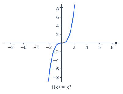
Drawn by us to help you understand the concept clearly, and verified to make sure it's accurate. For exams, practice from your textbook's own diagram.
The figure shows the graph of the function drawn on a standard Cartesian plane. The horizontal axis is the -axis (the domain, all real numbers), and the vertical axis is the -axis (the range, also all real numbers). The curve itself is an S-shaped cubic that passes through the origin . Near the origin the graph is very flat — it hugs the -axis for a short stretch — but as moves away from zero in either direction, the curve steepens dramatically and rises (or falls) without bound.
The key idea the figure teaches is that the cubic function is an odd function: it is symmetric about the origin. For every point on the graph, the point is also on the graph. This is why the curve goes through the origin and why the left-hand side is a mirror image of the right-hand side, but flipped upside down. The flatness near reflects the fact that for small , is much smaller than — for example, — so the graph barely rises. The steepness away from the origin shows that grows faster than any linear or quadratic function for large .
The central formula the textbook develops with this figure is simply the definition of the function itself:
Here is a real-valued function from to . The symbol represents any real number (the input), and is the output. The domain is all real numbers, and the range is also all real numbers — every real number has a real cube root, so the graph covers the entire vertical axis.
The textbook uses this figure as part of a sequence introducing basic polynomial functions. After the identity function (a straight line) and the square function (a parabola), the cube function is the next natural example. The figure makes the contrast clear: unlike the parabola (which is even and U-shaped), the cubic is odd and S-shaped, and unlike the identity line, it is not straight. …
Drawn by us to help you understand the concept clearly, and verified to make sure it's accurate. For exams, practice from your textbook's own diagram.
Fig. 2.12 shows the graph of the function , defined for all real numbers except . The axes are drawn in the usual way: a horizontal -axis and a vertical -axis, crossing at the origin. The curve consists of two separate branches, each drawn in indigo. One branch lies entirely in the first quadrant (where and ), and the other lies in the third quadrant (where and ). Both branches are smooth curves that get closer and closer to the -axis and the -axis but never touch or cross them — those axes are the asymptotes of the graph.
The physical idea the figure teaches is that is a reciprocal relationship: as grows large and positive, becomes very small and positive (the branch hugs the -axis far to the right). As approaches from the positive side, shoots upward without bound (the branch hugs the -axis near the top). The same behaviour repeats in the third quadrant but with both coordinates negative: as becomes large and negative, is a small negative number; as approaches from the negative side, plunges downward without bound. The graph is symmetric about the origin — if you rotate it , it lands on itself — which reflects the algebraic fact that .
The key formula the textbook develops with this figure is the definition of the function itself:
Here, denotes the set of all real numbers, and means all real numbers except . The domain of is because division by zero is undefined. The range is also : no matter what non-zero real number you pick, there is some that gives that (for example, comes from ), but is never achieved because can never equal zero.
A common mistake is to think the graph is continuous across . It is not — the function is undefined at , so the two branches are completely separate. The curve does not cross the -axis at any point. …
Drawn by us to help you understand the concept clearly, and verified to make sure it's accurate. For exams, practice from your textbook's own diagram.
The modulus function is defined piecewise because absolute value behaves differently for non‑negative and negative numbers. The definition is:
For every , the output is simply itself — so on the right half of the graph, the function follows the line . For every , the output is the positive opposite , which means the left half follows the line . Both are straight lines through the origin, one with slope and the other with slope .
The figure shows a standard Cartesian plane with the -axis horizontal and the -axis vertical. The graph is a single continuous V‑shaped curve. Its vertex sits exactly at the origin . From the vertex, the left arm rises into the second quadrant (where is negative, is positive) at a angle to the axes — that is the line . The right arm rises into the first quadrant (both and positive) also at — that is the line . The two arms are symmetric about the -axis.
The domain of the modulus function is all real numbers . The range is only non‑negative real numbers: . No matter what you plug in, is never negative.
The physical idea the graph teaches is that absolute value measures distance from zero on the number line. Distance is always non‑negative, and the graph’s V‑shape reflects that: as you move away from zero in either direction, the distance (the -value) increases at the same rate. The sharp corner at the origin is the key visual clue — the function changes its rule exactly at , and that point is the minimum value of the function.
A common mistake is to think the modulus function is the same as the identity function . They are identical only for . For negative , the identity function gives a negative output, while the modulus function flips the sign to give a positive output. The graph of is a single straight line through the origin; the graph of is a V‑shape. …
Drawn by us to help you understand the concept clearly, and verified to make sure it's accurate. For exams, practice from your textbook's own diagram.
The signum function is a simple but important piecewise-defined function that tells you the sign of a real number. Its formal definition is:
The domain is all real numbers , and the range is the three-point set .
What the graph shows. The figure plots on a standard Cartesian plane. For every positive , the output is exactly — so the graph is a horizontal ray along that starts just to the right of the origin and extends infinitely to the right. The starting point at is an open circle, because the function does not take the value at ; it takes there. An arrowhead on the right end of the ray indicates it continues without bound.
For every negative , the output is , giving a horizontal ray along that runs from the far left toward the origin. Again, the endpoint at is an open circle — the value is not assigned at . An arrowhead on the left end shows the ray extends to .
At the origin itself, the graph has a single filled dot at . This solid dot represents the third piece of the definition: . The open circles on the two rays and the filled dot at the origin together make the graph complete and unambiguous — they show exactly which -value belongs to each .
A common mistake is to connect the two rays or to draw a continuous line through the origin. The signum function is discontinuous at : the left-hand limit is , the right-hand limit is , but the actual value is . The open circles and the separate filled dot are the visual signal of this jump.
The key idea the figure teaches. The signum function is a piecewise constant function that compresses the entire real line into just three outputs. It is often used in later mathematics to express the sign of a quantity without caring about its magnitude. For example, the absolute value function can be written as , and the derivative of (for ) is .
This alternative form is useful: for , ; for , . It fails at because division by zero is undefined, which is why the piecewise definition is the complete one. …
![Fig. 2.15 — Graph of the greatest integer function f(x) = [x]](/figures/relations-and-functions-class-11/graph-greatest-integer-function-fig-2-15.svg)
Drawn by us to help you understand the concept clearly, and verified to make sure it's accurate. For exams, practice from your textbook's own diagram.
The figure shows the graph of the function , where denotes the greatest integer less than or equal to . The horizontal axis is labelled and runs from to ; the vertical axis is labelled and runs from to . The graph consists of seven horizontal step segments, each exactly one unit wide. Every segment is drawn in indigo.
For each integer , the segment corresponding to lies at height and covers the interval . The left endpoint of each segment — the point — is marked with a filled dot, indicating that the value is included at that . The right endpoint — the point — is marked with an open circle, indicating that the value is not attained at (because at , the greatest integer less than or equal to jumps to ). The graph therefore rises by one unit at every integer value of , creating a staircase that climbs to the right and descends to the left.
A common mistake is to think rounds to the nearest integer. It does not — it always takes the integer below (or equal to) . For negative numbers this matters: , not , because is the greatest integer less than or equal to .
The key idea the figure teaches is that the greatest integer function is a step function — it is constant on intervals between consecutive integers, and it jumps discontinuously at every integer. The filled and open dots make the left‑continuity of the function visible: at each integer , the function value is (the closed dot), but just to the right of the value is still until the next integer is reached.
…