Mathematics · Ch 4 — Straight Lines

Introduction

4.1

Introduction

9.1 Introduction

Coordinate geometry is the bridge between algebra and geometry. You have already encountered it in earlier classes — plotting points, finding distances, dividing line segments, and computing areas. What you may not have realised is that every geometric figure can be described by an equation, and every equation can be visualised as a geometric shape. This idea was revolutionised by the French philosopher and mathematician René Descartes in his 1637 work La Géométrie. Before Descartes, geometry was studied purely through diagrams and logical reasoning. After him, we could calculate geometry.

The chapter ahead focuses on the simplest geometric figure — the straight line. Despite its simplicity, the line appears everywhere: in the slope of a road, the path of a ray of light, the edge of a ruler, the graph of a linear equation. Our goal is to represent a line algebraically, and the key to that representation is the concept of slope.

But before we move to new ideas, we must revisit the foundations laid in earlier classes. The textbook opens with a quick recap of four fundamental formulae. Each one is essential; each one will be used repeatedly in the coming sections.

Recap of Coordinate Geometry Basics

Consider the XY-plane. Every point is located by an ordered pair $(x, y)$ . The $x$ -coordinate tells you the distance from the $y$ -axis (positive to the right, negative to the left), and the $y$ -coordinate tells you the distance from the $x$ -axis (positive upward, negative downward).

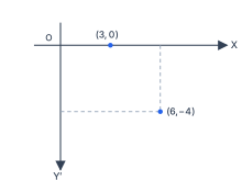
For example, the point $(6, -4)$ lies 6 units to the right of the $y$ -axis and 4 units below the $x$ -axis. The point $(3, 0)$ lies 3 units to the right of the $y$ -axis and exactly on the $x$ -axis (zero vertical distance).

With this understanding, we recall four key results.

I. Distance Between Two Points

Given two points $P(x_1, y_1)$ and $Q(x_2, y_2)$ , the distance between them is:

PQ = \sqrt{(x_2 - x_1)^2 + (y_2 - y_1)^2}

This formula is a direct application of the Pythagorean theorem. The horizontal separation is $|x_2 - x_1|$ , the vertical separation is $|y_2 - y_1|$ , and the straight-line distance is the hypotenuse of the right triangle they form.

Example: Find the distance between $(6, -4)$ and $(3, 0)$ .

PQ = \sqrt{(3 - 6)^2 + (0 - (-4))^2} = \sqrt{(-3)^2 + (4)^2} = \sqrt{9 + 16} = \sqrt{25} = 5 \text{ units}

Watch out

A common mistake is to forget the square root. The expression $\sqrt{(x_2 - x_1)^2 + (y_2 - y_1)^2}$ gives the distance; $(x_2 - x_1)^2 + (y_2 - y_1)^2$ alone gives the square of the distance.

II. Section Formula (Internal Division)

If a point $P$ divides the line segment joining $A(x_1, y_1)$ and $B(x_2, y_2)$ internally in the ratio $m : n$ (meaning $AP : PB = m : n$ ), then the coordinates of $P$ are:

P\left( \frac{m x_2 + n x_1}{m + n}, \frac{m y_2 + n y_1}{m + n} \right)

Notice the pattern: the coordinates of $B$ (the point towards which the division is measured) are multiplied by $m$ , and the coordinates of $A$ are multiplied by $n$ . The denominator is the sum $m + n$ .

Example: Find the point that divides the segment joining $A(1, -3)$ and $B(-3, 9)$ internally in the ratio $1 : 3$ .

Here $m = 1$ , $n = 3$ , $x_1 = 1$ , $y_1 = -3$ , $x_2 = -3$ , $y_2 = 9$ .

x = \frac{1(-3) + 3(1)}{1 + 3} = \frac{-3 + 3}{4} = \frac{0}{4} = 0

y = \frac{1(9) + 3(-3)}{1 + 3} = \frac{9 - 9}{4} = \frac{0}{4} = 0

So the point is $(0, 0)$ — the origin itself.

Tip

To remember which coordinate gets multiplied by $m$ and which by $n$ , think: the point $B$ is "farther" in the ratio $m$ , so its coordinates get the $m$ multiplier. The point $A$ is "closer" in the ratio $n$ , so its coordinates get the $n$ multiplier.

III. Midpoint Formula (Special Case of Section Formula)

When $m = n$ , the point divides the segment in the ratio $1 : 1$ , i.e., it is the midpoint. Substituting $m = n$ into the section formula gives:

\text{Midpoint} = \left( \frac{x_1 + x_2}{2}, \frac{y_1 + y_2}{2} \right)

This is simply the average of the $x$ -coordinates and the average of the $y$ -coordinates.

Important

The midpoint formula is a special case of the section formula. You do not need to memorise it separately — just remember that when $m = n$ , the ratio simplifies to $1:1$ , and the formula collapses to the average.

IV. Area of a Triangle

Given three vertices $A(x_1, y_1)$ , $B(x_2, y_2)$ , and $C(x_3, y_3)$ , the area of triangle $ABC$ is:

\text{Area} = \frac{1}{2} \left| x_1(y_2 - y_3) + x_2(y_3 - y_1) + x_3(y_1 - y_2) \right|

The absolute value ensures the area is positive. The expression inside the absolute value can be positive or negative depending on the order of the vertices; its magnitude gives twice the area.

Example: Find the area of the triangle with vertices $(4, 4)$ , $(3, -2)$ , and $(-3, 16)$ .

Let $(x_1, y_1) = (4, 4)$ , $(x_2, y_2) = (3, -2)$ , $(x_3, y_3) = (-3, 16)$ .

\begin{aligned} \text{Area} &= \frac{1}{2} \left| 4(-2 - 16) + 3(16 - 4) + (-3)(4 - (-2)) \right| \\ &= \frac{1}{2} \left| 4(-18) + 3(12) + (-3)(6) \right| \\ &= \frac{1}{2} \left| -72 + 36 - 18 \right| \\ &= \frac{1}{2} \left| -54 \right| = \frac{1}{2} \times 54 = 27 \text{ square units} \end{aligned}

Note

The formula works for any three points. If the three points are collinear (lie on the same straight line), the area comes out to zero. This gives us a quick algebraic test for collinearity: three points $A$ , $B$ , $C$ are collinear if and only if the area of triangle $ABC$ is zero.

What Lies Ahead

These four formulae — distance, section, midpoint, and area — are the tools you already possess. In this chapter, we will build upon them to study the straight line. The central new idea is slope, which measures the steepness and direction of a line. Once we have slope, we can write the equation of a line in several forms, find the angle between two lines, compute distances from a point to a line, and solve many practical problems.

The line may be the simplest geometric figure, but its algebraic treatment opens the door to a vast and beautiful landscape of analytical geometry.

Figure 9.1Points (3,0) and (6,−4) in the XY-plane

Fig. 9.1 — Points (3,0) and (6,−4) in the XY-plane

Drawn by us to help you understand the concept clearly, and verified to make sure it's accurate. For exams, practice from your textbook's own diagram.

The figure is a simple two-dimensional coordinate grid — the standard $XY$ -plane you have been using since Class 9. The axes are drawn with the origin $O$ at the centre. The $X$ -axis runs horizontally to the right (positive direction), and the $Y$ -axis runs vertically downward (the negative $Y$ direction is shown, since the point $(6,-4)$ lies below the $X$ -axis). The axes are labelled $X$ and $Y'$ respectively.

Two points are plotted. The first is $(3,0)$ : it lies directly on the $X$ -axis, three units to the right of the origin. The second is $(6,-4)$ : it is located six units to the right of the $Y$ -axis (along the positive $X$ direction) and four units below the $X$ -axis (along the negative $Y$ direction). To make this location clear, the figure includes dashed vertical and horizontal guide lines from $(6,-4)$ to the axes — a vertical dashed line drops straight down from the point to the $X$ -axis, and a horizontal dashed line runs leftwards from the point to the $Y$ -axis. These guide lines help you see that the $x$ -coordinate (6) is the perpendicular distance to the $Y$ -axis, and the $y$ -coordinate (-4) is the perpendicular distance to the $X$ -axis.

The entire purpose of this figure is to remind you of the fundamental idea of coordinate geometry: every point in the plane is uniquely identified by an ordered pair $(x,y)$ , where $x$ is the signed distance from the $Y$ -axis and $y$ is the signed distance from the $X$ -axis. The figure also sets the stage for the distance formula, which the textbook immediately applies to these two points.

\text{Distance between } P(x_1,y_1) \text{ and } Q(x_2,y_2) = \sqrt{(x_2 - x_1)^2 + (y_2 - y_1)^2}

Using the points from the figure — $P(3,0)$ and $Q(6,-4)$ — the distance is:

\sqrt{(6-3)^2 + (-4-0)^2} = \sqrt{3^2 + (-4)^2} = \sqrt{9+16} = \sqrt{25} = 5 \text{ units}.

The $5$ here is the straight-line length of the segment joining the two plotted points. The figure itself does not show this segment, but the formula is the key algebraic tool that the figure motivates: once you know the coordinates, you can compute the distance without measuring.

Watch out

A common mistake is to forget the parentheses when squaring the differences. Write $(x_2 - x_1)^2$ , not $x_2 - x_1^2$ . Also, the order inside the square does not matter: $(x_2 - x_1)^2 = (x_1 - x_2)^2$ .

The figure also implicitly reinforces the sign convention: the $y$ -coordinate of $(6,-4)$ is negative because the point lies below the $X$ -axis. The distance formula squares the difference, so the sign disappears — but the sign matters when you later compute slopes or use the section formula. For instance, the midpoint of $(3,0)$ and $(6,-4)$ is $\left( \frac{3+6}{2}, \frac{0+(-4)}{2} \right) = (4.5, -2)$ , which lies exactly halfway between them, below the $X$ -axis. The figure does not show this midpoint, but the coordinates follow directly from the plotted points.

In short, Fig. 9.1 is a visual anchor for the entire chapter: it shows how a pair of numbers pins down a location, and it provides the concrete example $(3,0)$ and $(6,-4)$ that the textbook uses to illustrate the distance formula, the section formula, and later the concept of slope. Whenever you see a new formula in this chapter, test it on these two points — it will help you connect the algebra to the geometry you see in the figure.

← Previous chapterCh 3 — Trigonometric Functions Next · 4.2 →Slope of a Line