Physics · Ch 10 — Thermal Properties of Matter

Thermal Expansion

10.5

Thermal Expansion

Most substances expand when heated and contract when cooled. This phenomenon — the change in size or volume of a material in response to a change in temperature — is called thermal expansion. It arises because the average kinetic energy of the atoms or molecules increases with temperature, causing them to vibrate more vigorously and, on average, occupy a larger volume.

The expansion is not the same in all directions for solids. For a solid rod, the increase in length is called linear expansion. For a sheet or plate, the increase in area is areal expansion (or superficial expansion). For a bulk solid or a liquid, the increase in volume is volumetric expansion (or cubical expansion). For isotropic solids (materials whose properties are the same in all directions), these three types of expansion are related by simple factors.

Note

Liquids and gases have no fixed shape, so only volumetric expansion is meaningful for them. Gases expand much more than liquids, and liquids expand more than solids, for the same temperature rise.

Linear Expansion

Consider a rod of length $L$ at some initial temperature $T$ . When the temperature changes by a small amount $\Delta T$ , the change in length $\Delta L$ is found experimentally to be directly proportional to both the original length $L$ and the temperature change $\Delta T$ . That is,

\Delta L \propto L \, \Delta T

Introducing a constant of proportionality $\alpha$ , called the coefficient of linear expansion, we write

\Delta L = \alpha \, L \, \Delta T

The coefficient $\alpha$ is defined as the fractional change in length per unit change in temperature:

\alpha = \frac{\Delta L}{L \, \Delta T}

Its SI unit is $\text{K}^{-1}$ (or $^\circ\text{C}^{-1}$ , since a change of 1 K equals a change of 1 $^\circ$ C). For most solids, $\alpha$ is a small positive number — typically of the order of $10^{-5} \, \text{K}^{-1}$ .

If the rod has length $L_0$ at temperature $T_0$ , and length $L$ at temperature $T$ , then $\Delta L = L - L_0$ and $\Delta T = T - T_0$ . The equation becomes

L - L_0 = \alpha \, L_0 \, (T - T_0)

L = L_0 \, [1 + \alpha (T - T_0)]

This is the working formula for linear expansion. It is accurate for small temperature changes; for very large $\Delta T$ , $\alpha$ itself may vary slightly with temperature.

Watch out

The formula $L = L_0 (1 + \alpha \Delta T)$ is an approximation valid when $\alpha \Delta T \ll 1$ . For large temperature changes, the exact differential relation $dL/dL = \alpha \, dT$ must be integrated, which may require knowing $\alpha(T)$ .

Table 10.1 Values of coefficient of linear expansion for some material

Material	$\alpha_l$ ( $10^{-5}\ \text{K}^{-1}$ )
Aluminium	2.5
Brass	1.8
Iron	1.2
Copper	1.7
Silver	1.9
Gold	1.4
Glass (pyrex)	0.32
Lead	0.29

Areal Expansion

For a two-dimensional object (a sheet or plate), the change in area $\Delta A$ for a temperature change $\Delta T$ is given by

\Delta A = \beta \, A \, \Delta T

where $\beta$ is the coefficient of areal expansion (or superficial expansion). Its definition is

\beta = \frac{\Delta A}{A \, \Delta T}

For an isotropic solid, $\beta$ is related to $\alpha$ by a simple factor. Consider a square plate of side $L$ at temperature $T_0$ . Its area is $A_0 = L_0^2$ . When heated to temperature $T$ , each side expands according to linear expansion:

L = L_0 (1 + \alpha \Delta T)

The new area is

A = L^2 = L_0^2 (1 + \alpha \Delta T)^2 = A_0 (1 + 2\alpha \Delta T + \alpha^2 \Delta T^2)

Since $\alpha$ is very small (typically $10^{-5}$ ), the term $\alpha^2 \Delta T^2$ is negligible compared to $2\alpha \Delta T$ for moderate $\Delta T$ . Hence

A \approx A_0 (1 + 2\alpha \Delta T)

Comparing with $A = A_0 (1 + \beta \Delta T)$ , we get

\beta = 2\alpha

Important

For isotropic solids, the coefficient of areal expansion is exactly twice the coefficient of linear expansion: $\beta = 2\alpha$ .

Volumetric Expansion

For a three-dimensional object, the change in volume $\Delta V$ for a temperature change $\Delta T$ is

\Delta V = \gamma \, V \, \Delta T

where $\gamma$ is the coefficient of volumetric expansion (or cubical expansion). Its definition is

\gamma = \frac{\Delta V}{V \, \Delta T}

For an isotropic solid, consider a cube of side $L_0$ at temperature $T_0$ , with volume $V_0 = L_0^3$ . After heating, each side becomes $L = L_0 (1 + \alpha \Delta T)$ , so the new volume is

V = L^3 = L_0^3 (1 + \alpha \Delta T)^3 = V_0 (1 + 3\alpha \Delta T + 3\alpha^2 \Delta T^2 + \alpha^3 \Delta T^3)

Neglecting terms of order $\alpha^2$ and higher (since $\alpha$ is very small), we get

V \approx V_0 (1 + 3\alpha \Delta T)

Comparing with $V = V_0 (1 + \gamma \Delta T)$ , we obtain

\gamma = 3\alpha

\alpha : \beta : \gamma = 1 : 2 : 3

›Proof

Derivation of $\gamma = 3\alpha$ for a rectangular block

Consider a rectangular block with sides $L_1$ , $L_2$ , $L_3$ at temperature $T_0$ . Its initial volume is $V_0 = L_1 L_2 L_3$ . After a temperature rise $\Delta T$ , each side expands linearly:

$L_1' = L_1 (1 + \alpha \Delta T), \quad L_2' = L_2 (1 + \alpha \Delta T), \quad L_3' = L_3 (1 + \alpha \Delta T)$

The new volume is

$V = L_1 L_2 L_3 (1 + \alpha \Delta T)^3 = V_0 (1 + 3\alpha \Delta T + 3\alpha^2 \Delta T^2 + \alpha^3 \Delta T^3)$

For $\alpha \Delta T \ll 1$ , the higher-order terms are negligible, so

$V \approx V_0 (1 + 3\alpha \Delta T)$

By definition, $V = V_0 (1 + \gamma \Delta T)$ , hence $\gamma = 3\alpha$ . This derivation holds for any shape because any volume can be thought of as composed of infinitesimal cubes, each expanding isotropically.

Table 10.2 Values of coefficient of volume expansion for some substances

Substance	$\alpha_v$ ( $\text{K}^{-1}$ )
Aluminium	$7 \times 10^{-5}$
Brass	$6 \times 10^{-5}$
Iron	$3.55 \times 10^{-5}$
Paraffin	$58.8 \times 10^{-5}$
Glass (ordinary)	$2.5 \times 10^{-5}$
Glass (pyrex)	$1 \times 10^{-5}$
Hard rubber	$2.4 \times 10^{-4}$
Invar	$2 \times 10^{-6}$
Mercury	$18.2 \times 10^{-5}$
Water	$20.7 \times 10^{-5}$
Alcohol (ethanol)	$110 \times 10^{-5}$

Thermal Expansion in Liquids

Liquids do not have a definite shape, so only volumetric expansion is considered. The coefficient of volumetric expansion for a liquid, $\gamma$ , is defined exactly as for solids:

\gamma = \frac{\Delta V}{V \, \Delta T}

However, when measuring the expansion of a liquid, the container itself expands. What we observe is the apparent expansion of the liquid — the difference between the actual expansion of the liquid and the expansion of the container. The real (or absolute) coefficient of volume expansion of the liquid, $\gamma_{\text{real}}$ , is related to the apparent coefficient, $\gamma_{\text{apparent}}$ , and the coefficient of volume expansion of the container material, $\gamma_{\text{container}}$ , by

\gamma_{\text{real}} = \gamma_{\text{apparent}} + \gamma_{\text{container}}

For example, if a liquid is placed in a glass vessel and heated, the liquid expands more than the glass. The observed rise in the liquid level corresponds to the apparent expansion. To find the true expansion of the liquid, the expansion of the glass must be added back.

Note

Water is an important exception to normal thermal expansion. Between $0^\circ\text{C}$ and $4^\circ\text{C}$ , water contracts when heated — it has a negative coefficient of expansion in this range. This anomalous behaviour is why ice floats and why lakes freeze from the top down.

Thermal Expansion in Gases

Gases expand much more than solids or liquids for the same temperature rise. For an ideal gas at constant pressure, the volume is directly proportional to the absolute temperature (Charles's law):

V \propto T \quad (\text{at constant pressure})

The coefficient of volume expansion for an ideal gas at constant pressure is

\gamma = \frac{1}{V} \left( \frac{\partial V}{\partial T} \right)_P = \frac{1}{T}

At $0^\circ\text{C}$ (273.15 K), this gives $\gamma = 1/273.15 \, \text{K}^{-1} \approx 3.66 \times 10^{-3} \, \text{K}^{-1}$ , which is about a hundred times larger than typical values for solids.

Watch out

The coefficient of expansion for a gas depends strongly on whether the pressure is held constant or the volume is held constant. The value $\gamma = 1/T$ applies only for constant-pressure processes. For constant-volume processes, the pressure coefficient is $\alpha_P = 1/T$ .

Applications and Consequences of Thermal Expansion

Thermal expansion has many practical implications:

Thermometers: Mercury or alcohol in a glass thermometer works because the liquid expands more than the glass.
Bimetallic strips: Two metals with different $\alpha$ values are bonded together. When heated, the strip bends because one side expands more than the other. This is used in thermostats and thermometers.
Expansion gaps: Bridges, railway tracks, and long pipelines have gaps or expansion joints to allow for expansion and contraction without buckling.
Tightening of nuts and bolts: A metal bolt can be heated to expand it, fitted into a hole, and then allowed to cool — it contracts and grips tightly.
Overhead power lines: Wires are hung with some slack to prevent snapping in cold weather when they contract.
Glass cookware: Borosilicate glass (Pyrex) has a very low $\alpha$ , so it does not crack when subjected to sudden temperature changes.

Tip

When solving problems, always check whether the given $\alpha$ is for linear expansion. If the problem involves area or volume, use $\beta = 2\alpha$ or $\gamma = 3\alpha$ respectively. For liquids, remember to account for container expansion if the problem asks for real expansion.

Thermal Stress: When Expansion Is Prevented

Thermal expansion assumes a body is free to expand or contract as its temperature changes. But what happens if a rod's ends are rigidly fixed, so it cannot expand at all when heated (or contract when cooled)? The material still "wants" to change length by the same $\Delta L = \alpha L \Delta T$ it would if free — but since the ends are fixed, an internal compressive (or tensile) strain develops instead of an actual change in length. This internal strain is accompanied by an internal stress, called thermal stress. …

Figure 10.5Thermal Expansion.

Drawn by us to help you understand the concept clearly, and verified to make sure it's accurate. For exams, practice from your textbook's own diagram.

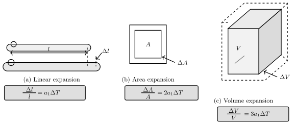
Fig. 10.5 is a single, clean illustration that shows how a solid expands in one, two, and three dimensions when its temperature rises. The figure is split into three panels, each showing the same physical idea: the change in size is proportional to the original size and to the temperature change.

Panel (a) shows a rod of original length $l$ . After heating by $\Delta T$ , its length becomes $l + \Delta l$ . The rod is drawn as a simple straight line or thin rectangle, with the increase $\Delta l$ clearly marked. The formula written alongside is $\frac{\Delta l}{l} = \alpha_1 \Delta T$ , where $\alpha_1$ is the coefficient of linear expansion. This tells you that the fractional change in length depends only on the material and the temperature rise, not on how long the rod was to begin with.

Panel (b) moves to two dimensions: a square of side $l$ expands to a larger square of side $l + \Delta l$ . The original area is $A = l^2$ , and the new area is $(l + \Delta l)^2$ . The figure shows the increase in both length and width, so the area increase $\Delta A$ is the sum of two strips along the edges plus a tiny corner square. The formula given is $\frac{\Delta A}{A} = 2\alpha_1 \Delta T$ . Notice that the factor 2 comes from the two independent directions — the linear expansion coefficient $\alpha_1$ applies to each side, so the area expansion coefficient is $2\alpha_1$ .

Panel (c) shows a cube of side $l$ expanding to a larger cube of side $l + \Delta l$ . The original volume is $V = l^3$ , and the new volume is $(l + \Delta l)^3$ . The formula is $\frac{\Delta V}{V} = 3\alpha_1 \Delta T$ . Again, the factor 3 comes from the three independent directions. The volume expansion coefficient is $3\alpha_1$ .

Important

The key insight of this figure is that for isotropic solids (materials that expand equally in all directions), the area and volume expansion coefficients are simple multiples of the linear coefficient: $\beta = 2\alpha$ and $\gamma = 3\alpha$ , where $\alpha = \alpha_1$ . These relations hold only when $\alpha \Delta T \ll 1$ , which is almost always true for solids.

The figure does not show any axes or curves — it is a schematic diagram, not a graph. Each panel is a before-and-after sketch of the same object, with the expansion exaggerated so you can see it clearly. The labels $\Delta l/l$ , $\Delta A/A$ , and $\Delta V/V$ are the fractional changes, and the formulas are written directly on the panels.

Watch out

A common mistake is to think that $\Delta A/A = 2\alpha \Delta T$ means the area expansion coefficient is $2\alpha$ only for a square. It is true for any shape, because area expansion depends on two perpendicular directions. The square is just the simplest shape to draw. …

Figure 10.6Coefficient of volume expansion of copper as a function of temperature.

Fig. 10.6 — Coefficient of volume expansion of copper as a function of temperature.

Drawn by us to help you understand the concept clearly, and verified to make sure it's accurate. For exams, practice from your textbook's own diagram.

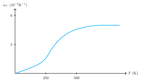
The figure plots the coefficient of volume expansion of copper, $\alpha_v$ , against absolute temperature $T$ (in kelvin). The vertical axis shows $\alpha_v$ in units of $10^{-5}\,\text{K}^{-1}$ , with tick marks at $3$ and $6$ on that scale. The horizontal axis is temperature, running from $250\,\text{K}$ to $500\,\text{K}$ .

The curve itself is sigmoid — it rises slowly at first, then more steeply through the middle range, and finally flattens off at the highest temperatures. This shape tells you that copper’s volume expansion coefficient is not constant; it depends strongly on temperature, especially in the range between roughly $300\,\text{K}$ and $450\,\text{K}$ . At low temperatures (near $250\,\text{K}$ ) the coefficient is small, meaning the material expands very little per degree rise. As the temperature increases, $\alpha_v$ grows, and the expansion per degree becomes larger. Above about $500\,\text{K}$ , the curve levels out — the coefficient approaches a nearly constant, high value.

The physical idea is straightforward: the atoms in a solid vibrate more as temperature rises, and the average distance between them increases. At very low temperatures, quantum effects keep the vibrations small, so the expansion coefficient is small. As the temperature climbs, the vibrations become larger and more anharmonic, causing the expansion coefficient to increase. At sufficiently high temperatures, the vibrations are so large that the material behaves almost like a classical solid, and $\alpha_v$ saturates to a constant value.

The textbook uses this figure to introduce the definition of the coefficient of volume expansion:

\alpha_v = \frac{1}{V} \frac{dV}{dT}

Here $V$ is the volume of the solid, $T$ is the absolute temperature, and $\frac{dV}{dT}$ is the rate of change of volume with temperature. The coefficient $\alpha_v$ tells you the fractional change in volume per unit temperature change. For a small temperature change $\Delta T$ , the volume change is approximately $\Delta V = \alpha_v V \Delta T$ .

The figure demonstrates that $\alpha_v$ is not a constant for copper — it varies with temperature. This is why the textbook plots it as a function of $T$ rather than giving a single number. For most practical calculations over a narrow temperature range, you can take an average value, but the graph shows the full story. …

Figure 10.7Thermal expansion of water.

Drawn by us to help you understand the concept clearly, and verified to make sure it's accurate. For exams, practice from your textbook's own diagram.

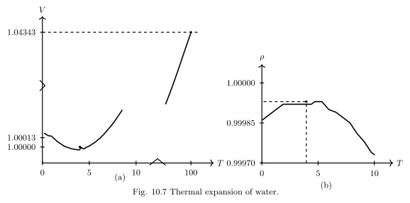
The figure has two panels that tell one story: water does not behave like most substances when heated.

Panel (a) plots volume of 1 kg of water (vertical axis) against temperature (horizontal axis, from 0 °C upward). The curve falls as temperature rises from 0 °C, reaches a clear minimum at 4 °C, then rises steadily. That minimum is the key: at 4 °C, 1 kg of water occupies its smallest volume.

Panel (b) plots density (vertical axis) against the same temperature axis. Density is mass divided by volume, so where volume is smallest, density is largest. The curve in panel (b) rises from 0 °C, peaks sharply at 4 °C, then falls. The peak density of water is $1000\ \text{kg m}^{-3}$ at 4 °C.

Important

Water contracts when heated from 0 °C to 4 °C, and expands only above 4 °C. This anomalous behaviour is why ice floats and why lakes freeze from the top down.

The physics behind the figure is the definition of density:

\rho = \frac{m}{V}

where $\rho$ is density, $m$ is mass (here 1 kg, constant), and $V$ is volume. Since mass is fixed, density and volume are inversely related — the minimum in panel (a) corresponds exactly to the maximum in panel (b).

The textbook uses this figure to introduce the coefficient of volume expansion $\gamma$ , defined as the fractional change in volume per unit change in temperature:

\gamma = \frac{1}{V} \frac{\Delta V}{\Delta T}

Here $\Delta V$ is the change in volume, $\Delta T$ the change in temperature, and $V$ the original volume. For most solids and liquids, $\gamma$ is positive and roughly constant over small temperature ranges. But for water between 0 °C and 4 °C, $\gamma$ is negative — the volume decreases as temperature increases. Above 4 °C, $\gamma$ becomes positive again.

Watch out

Never apply the formula $\Delta V = \gamma V \Delta T$ across the 0–4 °C range for water. The sign of $\gamma$ changes, so the linear approximation fails. The figure shows the actual non-linear behaviour. …

Figure 10.8Fig. 10.8

Drawn by us to help you understand the concept clearly, and verified to make sure it's accurate. For exams, practice from your textbook's own diagram.

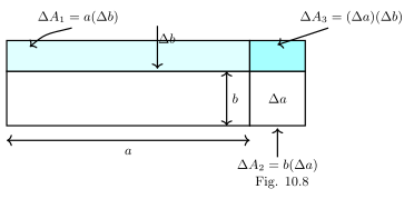
The figure shows a rectangular sheet of material with original length $a$ and breadth $b$ . When the sheet is heated, it expands uniformly in both directions. The diagram breaks this expansion into three distinct regions drawn on the expanded sheet.

Along the right side, a vertical strip of width $\Delta a$ runs the full original height $b$ . This strip represents the increase in length: its area is $\Delta A_2 = b(\Delta a)$ . Along the top, a horizontal strip of height $\Delta b$ runs the full original length $a$ , representing the increase in breadth: its area is $\Delta A_1 = a(\Delta b)$ . In the top-right corner, a small rectangle of dimensions $\Delta a$ by $\Delta b$ sits where the two strips meet. Its area is $\Delta A_3 = (\Delta a)(\Delta b)$ .

The total change in area of the sheet is the sum of these three contributions:

\Delta A = a(\Delta b) + b(\Delta a) + (\Delta a)(\Delta b)

This is the physical idea the figure teaches: area expansion is not simply two independent stretches. The corner piece $\Delta A_3$ is a second-order term — it is the product of two small increments. For small temperature changes, $\Delta a$ and $\Delta b$ are themselves small, so their product is much smaller than the other two terms. The textbook uses this geometric picture to derive the formula for area expansion.

\Delta A = A_0 \, \alpha \, \Delta T

The derivation follows from the figure. Since $\Delta a = a \, \alpha \, \Delta T$ and $\Delta b = b \, \alpha \, \Delta T$ , substitute into the expression for $\Delta A$ :

\Delta A = a(b \, \alpha \, \Delta T) + b(a \, \alpha \, \Delta T) + (a \, \alpha \, \Delta T)(b \, \alpha \, \Delta T)

The first two terms give $2ab \, \alpha \, \Delta T = 2A_0 \, \alpha \, \Delta T$ . The third term is $ab \, \alpha^2 (\Delta T)^2 = A_0 \, \alpha^2 (\Delta T)^2$ . For typical temperature changes, $\alpha$ is of order $10^{-5} \, \text{K}^{-1}$ , so $\alpha^2 (\Delta T)^2$ is negligible compared to $2\alpha \, \Delta T$ . Hence the area expansion coefficient is $2\alpha$ , and the formula reduces to $\Delta A = A_0 (2\alpha) \Delta T$ . …

Start your 14-day free trial to unlock the full solution →

← Previous · 10.4Ideal-gas Equation and Absolute Temperature Next · 10.5 →Example 10.1 — Show that the coefficient of area expansion, (Δ A/A)/Δ T, of a rectang…