Variation of Conductivity and Molar Conductivity with Concentration

Both conductivity and molar conductivity change as the concentration of an electrolyte changes. Conductivity always decreases with dilution, for weak and strong electrolytes alike — this is simply because the number of ions per unit volume available to carry the current falls as the solution is made more dilute.

Recall that conductivity is the conductance of a unit volume of solution held between electrodes of unit area and unit separation, so that $\kappa = G$ when $A$ and $l$ are both unity. Molar conductivity, by contrast, is the conductance of the volume $V$ of solution that contains exactly one mole of the electrolyte, held between electrodes of unit separation:

Molar conductivity increases with dilution. This looks like the opposite behaviour of $\kappa$, and it is: as a solution is diluted, the volume $V$ that contains one mole of electrolyte keeps growing, and the drop in $\kappa$ turns out to be more than compensated by this growth in $V$. Equivalently, $\Lambda_m$ at a given concentration can be pictured as the conductance of the electrolytic solution between the electrodes of a conductivity cell held one unit distance apart, but with the electrode area made just large enough to hold the entire volume of solution containing one mole of electrolyte.

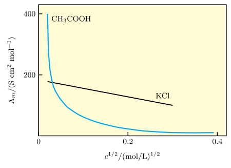
As concentration is lowered all the way toward zero, molar conductivity approaches a ceiling value called the limiting molar conductivity, written $\Lambda_m^0$. How $\Lambda_m$ climbs toward this ceiling, though, looks quite different for strong and weak electrolytes — the two are compared directly on a plot of $\Lambda_m$ against $\sqrt{c}$ in the accompanying figure card, which contrasts a strong electrolyte (KCl) with a weak one (acetic acid); refer to that figure rather than re-describing its curves here.

Strong Electrolytes

For a strong electrolyte, $\Lambda_m$ increases only slowly as the solution is diluted, and this rise is well described by:

$\Lambda_m^0$ — limiting molar conductivity (value at infinite dilution)

$A$ — a positive constant

$c$ — concentration

Plotting $\Lambda_m$ against $\sqrt{c}$ gives a near-straight line whose intercept is $\Lambda_m^0$ and whose slope is $-A$. This is precisely why $\Lambda_m^0$ for a strong electrolyte can be obtained by extrapolating the plot back to $\sqrt{c} = 0$.

The constant $A$, for a given solvent and temperature, depends on the valence type of the electrolyte — that is, on the charges carried by the cation and anion it dissociates into. NaCl, CaCl₂ and MgSO₄, for instance, are described as 1-1, 2-1 and 2-2 electrolytes respectively, and every electrolyte of a given valence type shares the same value of $A$.

Kohlrausch's regularity. Examining $\Lambda_m^0$ values across many strong electrolytes, Kohlrausch noticed that the difference between the limiting molar conductivities of a sodium salt and the corresponding potassium salt (same anion X in both) stays nearly constant, no matter which anion X is chosen. At 298 K, for example:

$\Lambda_m^{0}(\text{KCl}) - \Lambda_m^{0}(\text{NaCl}) = \Lambda_m^{0}(\text{KBr}) - \Lambda_m^{0}(\text{NaBr}) = \Lambda_m^{0}(\text{KI}) - \Lambda_m^{0}(\text{NaI}) \simeq 23.4\ \text{S cm}^2\,\text{mol}^{-1}$ The same kind of near-constant difference shows up when comparing other matched pairs of salts that share one common ion. For instance:

$\Lambda_m^{0}(\text{NaBr}) - \Lambda_m^{0}(\text{NaCl}) = \Lambda_m^{0}(\text{KBr}) - \Lambda_m^{0}(\text{KCl}) \simeq 1.8\ \text{S cm}^2\,\text{mol}^{-1}$ This regularity is the clue that each ion is contributing its own fixed, independent share to the total conductivity — a cation's contribution does not depend on which anion happens to be paired with it, and vice versa.

Kohlrausch's law of independent migration of ions. This observation was generalised into a law: the limiting molar conductivity of an electrolyte can be expressed as the sum of the individual contributions of its cation and its anion. For sodium chloride, for instance, this reads

$\Lambda_m^{0}(\text{NaCl}) = \lambda_{\text{Na}^+}^{0} + \lambda_{\text{Cl}^-}^{0}$ For an electrolyte that dissociates to give $\nu_+$ cations and $\nu_-$ anions:

$\lambda_+^0,\ \lambda_-^0$ — the limiting molar conductivities of the cation and anion respectively (each ion's own fixed contribution at infinite dilution)

$\nu_+,\ \nu_-$ — the number of cations and anions produced per formula unit of the electrolyte on dissociation

A reference table listing $\lambda^0$ values for a range of common cations and anions in water is provided as a separate card; it supplies exactly the per-ion numbers this equation needs and is not reproduced in the text here.

Why this law matters. It lets $\Lambda_m^0$ be computed for essentially any electrolyte purely by adding up tabulated single-ion values — including, crucially, for an electrolyte whose own $\Lambda_m^0$ cannot be measured directly by extrapolation at all, which is exactly the situation with weak electrolytes below.

Weak Electrolytes

Weak electrolytes, such as acetic acid, are only partly dissociated, and their degree of dissociation is lower at higher concentrations. So as such a solution is diluted, $\Lambda_m$ rises for two reasons at once: fewer interionic interactions (as with strong electrolytes) and a rising degree of dissociation, which puts more ions into circulation per mole of electrolyte present. The combined effect is that $\Lambda_m$ shoots up steeply on dilution, particularly at the lower end of the concentration range, rather than climbing gently the way a strong electrolyte's does.

This steep, non-linear rise means the $\Lambda_m$ vs $\sqrt{c}$ plot for a weak electrolyte does not settle into a straight line running to a clean intercept, so $\Lambda_m^0$ cannot be read off by extrapolating it to zero concentration. At infinite dilution the electrolyte would in principle dissociate completely ($\alpha = 1$), but by that point the solution's conductivity is too low to be measured with any accuracy — so that limit can never actually be approached experimentally. Instead, $\Lambda_m^0$ for a weak electrolyte has to be obtained indirectly, by applying Kohlrausch's law of independent migration of ions (building it up from ionic contributions, or from combinations of strong electrolytes sharing the relevant ions).

Degree of Dissociation and the Dissociation Constant …