Chemistry · Ch 4 — Chemical Bonding and Molecular Structure

Valence Bond Theory

4.5

Valence Bond Theory

4.5 Valence Bond Theory

The Lewis approach gives us a way to write the structure of a molecule, but it cannot explain why a chemical bond forms in the first place. It also offers no reason for the very different bond dissociation enthalpies and bond lengths seen in molecules like H₂ (435.8 kJ mol⁻¹, 74 pm) and F₂ (155 kJ mol⁻¹, 144 pm), even though both involve a single covalent bond formed by sharing one electron pair. The VSEPR theory, while useful for predicting the geometry of simple molecules, does not provide a theoretical explanation for those shapes and has limited scope.

To overcome these shortcomings, two quantum-mechanical theories were developed: valence bond (VB) theory and molecular orbital (MO) theory. VB theory was introduced by Heitler and London in 1927 and later expanded by Pauling and others. It builds on the concepts of atomic orbitals, electronic configurations, the overlap of atomic orbitals, hybridization, and the principles of variation and superposition. A full mathematical treatment is beyond the scope of this book, so we will discuss VB theory in a qualitative, non-mathematical way.

Formation of the Hydrogen Molecule

Let us consider the simplest case: two hydrogen atoms, A and B, approaching each other. Atom A has a nucleus Nₐ and an electron eₐ; atom B has a nucleus N_B and an electron e_B.

When the atoms are far apart, there is no interaction between them. As they come closer, new forces begin to act.

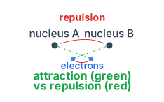
Attractive forces arise between:

the nucleus of one atom and its own electron (Nₐ–eₐ and N_B–e_B)
the nucleus of one atom and the electron of the other atom (Nₐ–e_B, N_B–eₐ)

Repulsive forces arise between:

the electrons of the two atoms (eₐ–e_B)
the nuclei of the two atoms (Nₐ–N_B)

Figure 4.7Forces of attraction and repulsion during the formation of an H₂ molecule.

Fig. 4.7 — Forces of attraction and repulsion during the formation of an H₂ molecule.

Drawn by us to help you understand the concept clearly, and verified to make sure it's accurate. For exams, practice from your textbook's own diagram.

Fig. 4.7 is a forces schematic, not a graph. It shows the two hydrogen nuclei (A and B) with the two electrons between and below them, and marks every new interaction that switches on as the atoms approach:

Attractive forces (green, dashed): each nucleus pulls on the other atom's electron — nucleus A on electron B and nucleus B on electron A. (Each nucleus of course also holds its own electron, as in the isolated atoms.)
Repulsive forces (red): the two electrons repel each other, and the two nuclei repel each other.

Whether a bond forms is a contest between these two sets. Experimentally, as two hydrogen atoms approach, the new attractions outweigh the new repulsions, so the system's potential energy falls and the atoms keep closing in — until, at 74 pm, attraction and repulsion balance and the energy bottoms out (that energy story is Fig. 4.8's).

Important

A bond is not a thing that "holds" atoms — it is the net result of electrostatics: electron density concentrated between two nuclei attracts both of them inward more strongly than the nucleus–nucleus and electron–electron repulsions push apart. …

Attractive forces pull the atoms together; repulsive forces push them apart. Experimentally, it is found that the magnitude of the new attractive forces is greater than that of the new repulsive forces. As a result, the two atoms move closer, and the potential energy of the system decreases.

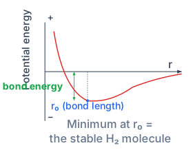
Eventually, a stage is reached where the net attractive force exactly balances the net repulsive force. At this point, the system has minimum energy. The two hydrogen atoms are now bonded together to form a stable H₂ molecule with a bond length of 74 pm.

Note

The energy released when the bond forms is called the bond enthalpy. For H₂, this is 435.8 kJ mol⁻¹. Conversely, 435.8 kJ of energy is required to break one mole of H₂ molecules into isolated hydrogen atoms:

$\text{H}_2(g) + 435.8\ \text{kJ mol}^{-1} \rightarrow \text{H}(g) + \text{H}(g)$ …

Figure 4.8The potential-energy curve for the formation of an H₂ molecule vs internuclear distance.

Fig. 4.8 — The potential-energy curve for the formation of an H₂ molecule vs internuclear distance.

Drawn by us to help you understand the concept clearly, and verified to make sure it's accurate. For exams, practice from your textbook's own diagram.

The figure plots potential energy (in kJ mol⁻¹) on the vertical axis against internuclear distance (in pm) on the horizontal axis. At very large separations — effectively infinite distance — the two hydrogen atoms do not interact, and the potential energy is taken as zero. As the atoms approach each other, the curve drops below zero, indicating that the system becomes more stable. The energy continues to fall until it reaches a single, well-defined minimum. That minimum occurs at an internuclear distance of 74 pm and corresponds to a potential energy of −435.8 kJ mol⁻¹. This is the bond length of H₂ and its bond dissociation enthalpy (the energy released when the bond forms, or the energy required to break it). Beyond that point — if the atoms are pushed even closer together — the curve rises steeply and sharply, reflecting the strong repulsion between the two positively charged nuclei when they are forced into the same small space.

The key physical idea is that a chemical bond is not a rigid stick connecting two atoms. It is a balance between attraction and repulsion. At large separations, attraction dominates as the electron cloud of one atom begins to be drawn toward the nucleus of the other. At very short separations, nuclear repulsion dominates. The equilibrium bond length is the distance at which these two opposing forces exactly cancel, giving the lowest possible energy for the system. That minimum is the most stable state of the molecule.

Important

The depth of the potential well (−435.8 kJ mol⁻¹) equals the bond dissociation energy of H₂. The position of the minimum (74 pm) is the equilibrium bond length. Both are experimentally measurable quantities.

The curve defines the quantity chemists care about most here — the bond dissociation energy:

D_0 = E(R_e) - E(\infty)

Here, $D_0$ is the bond dissociation energy (the energy required to break the bond at 0 K), $E(R_e)$ is the potential energy at the equilibrium bond length $R_e$ (the minimum of the curve), and $E(\infty)$ is the potential energy when the atoms are infinitely far apart (taken as zero). For H₂, $D_0 = 435.8\ \text{kJ mol}^{-1}$ and $R_e = 74\ \text{pm}$ .

A second, more detailed formula that the figure helps to motivate is the Morse potential, which approximates the shape of the curve:

V(r) = D_e \left[ 1 - e^{-a(r - r_e)} \right]^2

In this equation, $V(r)$ is the potential energy at internuclear distance $r$ , $D_e$ is the depth of the potential well (the dissociation energy measured from the minimum, not from zero-point energy), $r_e$ is the equilibrium bond length, and $a$ is a constant that controls the width of the well (related to the force constant of the bond). The Morse potential captures the essential features: a flat approach at large $r$ , a smooth minimum at $r = r_e$ , and a steep repulsive wall at small $r$ .

Watch out

Do not confuse $D_e$ (the depth from the minimum to the dissociation limit) with $D_0$ (the actual bond dissociation energy). $D_0$ is slightly smaller than $D_e$ because the molecule always has some zero-point vibrational energy, even at 0 K. The figure’s minimum is at $E = -435.8$ kJ mol⁻¹, which is $D_0$ for H₂, not $D_e$ .

The figure also implicitly teaches that the bond is not a static thing. The molecule vibrates — the atoms oscillate back and forth around the equilibrium distance $r_e$ , like a ball rolling in a bowl. The shape of the curve near the minimum determines the vibrational frequency. A steeper curve (larger $a$ in the Morse potential) means a stiffer bond and a higher vibrational frequency. A shallower curve means a weaker bond and a lower frequency. …

Start your 14-day free trial to unlock the full solution →

← Previous · 4.4The Valence Shell Electron Pair Repulsion (VSEPR) Theory Next · 4.5.1 →Orbital Overlap Concept