Biology · Ch 11 — Organisms and Populations
Population Growth
Population Growth
A population's size is never fixed. It rises and falls constantly because of changes in food availability, predation pressure, and weather. Tracking these changes in density tells us whether a population is flourishing or declining.
Four basic processes drive all fluctuations in population density. Two of them increase density, and two decrease it.
- Natality – the number of births in a given period, added to the initial density.
- Immigration – the number of individuals of the same species that enter the habitat from elsewhere during the time period.
- Mortality – the number of deaths in the population during the given period.
- Emigration – the number of individuals that leave the habitat and go elsewhere during the time period.
If we let N be the population density at time t, then the density at time t+1 is:
Nt+1 = Nt + [(B + I) - (D + E)]
Population density increases when births plus immigrants (B + I) exceed deaths plus emigrants (D + E). Under normal conditions, births and deaths are the most important factors. Immigration and emigration become significant only in special situations — for example, when a new habitat is being colonised, immigration can contribute more to growth than birth rates do.
Growth Models
Does population growth follow a predictable pattern? Human population growth is a major concern, and it is natural to ask whether other animal populations grow without restraint or show limits. Nature may offer lessons on controlling growth.
Exponential Growth
For unimpeded growth, resources (food and space) must be unlimited. Under ideal conditions, every species can realise its full innate potential to increase in number — as Darwin observed while developing his theory of natural selection. The population then grows in an exponential or geometric fashion.
If N is the population size, b is the per capita birth rate, and d is the per capita death rate, then the change in N per unit time is:
dN/dt = (b - d) × N
Let (b - d) = r. Then:
dN/dt = rN
Here, r is called the intrinsic rate of natural increase. It is a key parameter for assessing the impact of any biotic or abiotic factor on population growth. To give you an idea of r values: for the Norway rat it is 0.015, for the flour beetle it is 0.12, and for the human population in India in 1981 it was 0.0205.
The integral form of this equation is:
Nt = N0 × e^(rt)
where Nt is population density after time t, N0 is density at time zero, r is the intrinsic rate of natural increase, and e is the base of natural logarithms (approximately 2.71828).
When plotted with N against time, exponential growth produces a J-shaped curve. Any species growing exponentially under unlimited resources can reach enormous densities in a short time. Darwin showed that even a slow-breeding animal like the elephant could reach huge numbers in the absence of checks.
A famous anecdote illustrates this dramatically. A king and his minister played chess. The minister said that if he won, he wanted wheat grains placed on the chessboard: one grain on square 1, two on square 2, four on square 3, eight on square 4, and so on, doubling each time for all 64 squares. The king agreed, thinking it a trivial bet. But by the time he reached halfway, he realised that all the wheat in his entire kingdom would not be enough to fill the 64 squares. Similarly, a single Paramecium dividing by binary fission every day would reach a mind-boggling population in 64 days — if food and space remained unlimited.
Logistic Growth
No population in nature has unlimited resources. Limited resources lead to competition among individuals. Eventually, only the fittest survive and reproduce. Many governments have also recognised this and introduced restraints to limit human population growth. …
Drawn by us to help you understand the concept clearly, and verified to make sure it's accurate. For exams, practice from your textbook's own diagram.
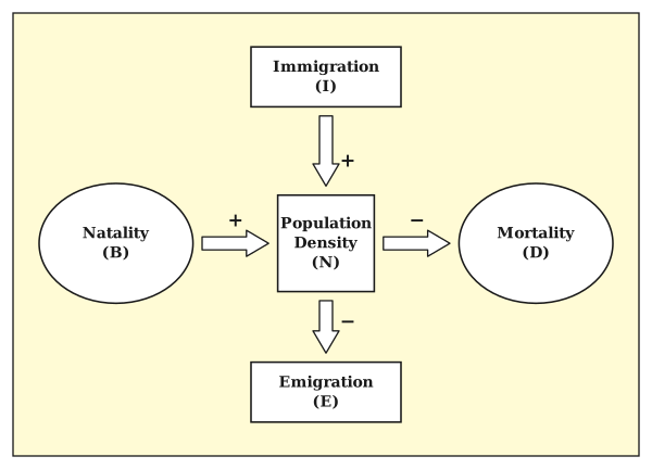
Figure 11.2 is a simple schematic that shows the four processes controlling population density. At the centre of the diagram is a box representing the population at a given time. Two arrows point inward, labelled Natality (B) and Immigration (I) — these add individuals to the population. Two arrows point outward, labelled Mortality (D) and Emigration (E) — these remove individuals. The diagram is built around the equation:
Nt+1 = Nt + [(B + I) - (D + E)]
where Nt is the population density at time t, and Nt+1 is the density one time unit later. The inward arrows increase N, the outward arrows decrease it, and the net change is the difference between the two sums. …
Drawn by us to help you understand the concept clearly, and verified to make sure it's accurate. For exams, practice from your textbook's own diagram.
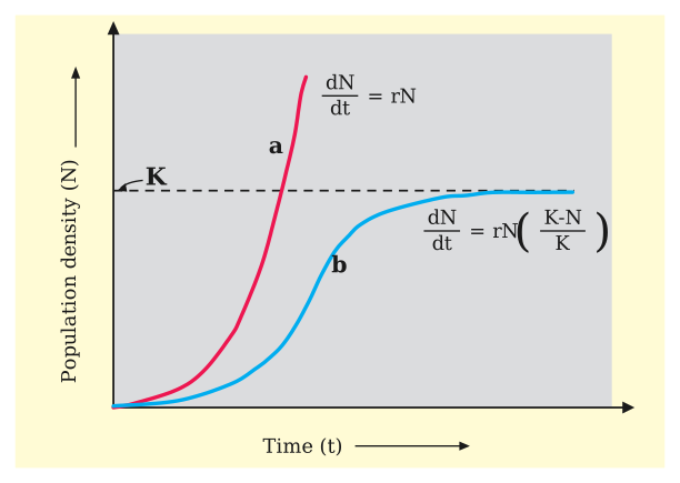
Figure 11.3 is a single graph with two curves, both plotting population density (N) on the vertical axis against time (t) on the horizontal axis. The graph is designed to contrast two fundamentally different growth patterns.
Curve (a) is labelled "Exponential" and is drawn as a J-shaped curve. It starts near the origin, rises slowly at first, then bends upward ever more steeply, with no upper limit shown. This curve represents what happens when resources are not limiting — the population grows at a rate proportional to its current size, so the larger it gets, the faster it grows. The curve has no horizontal asymptote; it simply keeps climbing.
Curve (b) is labelled "Logistic" and is drawn as an S-shaped (sigmoid) curve. It also starts near the origin, but its shape is very different. It begins with a shallow, nearly flat region — the lag phase — where growth is slow. Then it enters a steep, nearly linear acceleration phase where growth is rapid. After that, the curve bends over and flattens out, entering a deceleration phase until it finally becomes horizontal. A dashed horizontal line runs across the graph at the level where curve (b) flattens out; this line is labelled K, the carrying capacity. The curve never crosses this line; it approaches it as an asymptote. …