Economics · Ch 4 — The Theory of the Firm under Perfect Competition

Condition 2

4.3.2

Condition 2

Why the Marginal Cost Curve Must Slope Upward at the Profit-Maximising Output

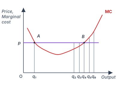
The second condition for profit maximisation under perfect competition deals with the shape of the marginal cost (MC) curve at the chosen output level. Even if price equals marginal cost, that output may not be the best choice. The textbook makes this point using Figure 4.3, which shows two output levels — $q_1$ and $q_4$ — where the market price equals marginal cost. At $q_1$ , however, the MC curve is sloping downward. The claim is that $q_1$ cannot be a profit-maximising output.

Figure 4.3Conditions 1 and 2 for profit maximisation. The figure demonstrates that when the market price is p, the profit-maximising firm cannot be q₁ (MC downward sloping), q₂ and q₃ (market price exceeds marginal cost), or q₅ and q₆ (marginal cost exceeds market price).

Fig. 4.3 — Conditions 1 and 2 for profit maximisation. The figure demonstrates that when the market price is p, the profit-maximising firm cannot be q₁ (MC downward sloping), q₂ and q₃ (market price exceeds marginal cost), or q₅ and q₆ (marginal cost exceeds market price).

Drawn by us to help you understand the concept clearly, and verified to make sure it's accurate. For exams, practice from your textbook's own diagram.

The figure plots the market price as a horizontal line against the firm’s marginal cost (MC) curve, which is U-shaped. The vertical axis measures price and cost (in rupees), the horizontal axis measures the firm’s output (in units). The market price $p$ is given — the firm cannot influence it. The MC curve first falls, reaches a minimum, then rises.

The figure shows six candidate output levels: $q_1$ , $q_2$ , $q_3$ , $q_4$ , $q_5$ , and $q_6$ . At $q_1$ , the MC curve is still sloping downward. At $q_2$ and $q_3$ , the MC curve lies below the price line — meaning the cost of producing one more unit is less than the revenue it brings. At $q_5$ and $q_6$ , the MC curve lies above the price line — the cost of an extra unit exceeds its revenue. Only at $q_4$ does the MC curve cross the price line from below, and at that point MC is rising.

The physical idea is simple: a firm maximises profit by producing the quantity where the cost of the last unit equals the price it fetches, provided that cost is increasing at that point. If MC is below price, the firm can raise profit by expanding output (each extra unit adds more to revenue than to cost). If MC is above price, the firm should cut output (the last unit cost more than it earned). The sweet spot is where MC equals price and is rising — that is the profit-maximising condition.

P = MC \quad \text{and} \quad MC \text{ is rising}

Here $P$ is the market price (the firm’s marginal revenue under perfect competition), and $MC$ is the firm’s marginal cost. The “rising” part is the second-order condition: it ensures the firm is at a maximum, not a minimum, of profit.

The textbook uses this figure to show why the firm cannot stop at $q_1$ , $q_2$ , $q_3$ , $q_5$ , or $q_6$ . At $q_1$ , MC is falling — if the firm produced one more unit, MC would be lower, so the equality $P = MC$ would not hold at a rising portion. At $q_2$ and $q_3$ , $P > MC$ , so profit increases with output. At $q_5$ and $q_6$ , $P < MC$ , so profit increases by reducing output. Only $q_4$ satisfies both conditions: $P = MC$ and MC is rising. …

Why? Consider any output level slightly to the left of $q_1$ . At those smaller outputs, the market price is lower than the marginal cost. The reasoning from section 4.3.1 tells us that when price is less than marginal cost, reducing output raises profit. So if the firm produces a little less than $q_1$ , its profit will be higher than at $q_1$ itself. That means $q_1$ is not the best choice — the firm can do better by moving left.

Watch out

A common mistake is to think that any point where $P = MC$ is automatically profit-maximising. That is only half the story. The MC curve must also be rising at that point. If MC is falling, the equality is a profit-minimising point instead.

The Intuition Behind the Upward-Sloping Requirement

The logic is symmetric. At $q_1$ , the MC curve is falling. For outputs just to the right of $q_1$ , marginal cost is lower than the price. The same section 4.3.1 argument says that when price exceeds marginal cost, increasing output raises profit. So the firm could also increase profit by moving to the right of $q_1$ . In other words, $q_1$ is a point where the firm can improve its profit by moving in either direction — left or right. That is the hallmark of a local minimum of profit, not a maximum.

The only way a point where $P = MC$ can be a true maximum is if the MC curve is rising at that point. When MC is rising, moving left (to a smaller output) means MC is lower than price, so profit would fall; moving right means MC is higher than price, so profit would also fall. That is the behaviour of a peak — the firm is stuck at the best possible output.

The Two Conditions Together

For a positive profit-maximising output under perfect competition, two conditions must hold simultaneously:

Price equals marginal cost — $P = MC$ .
Marginal cost must be rising at that output — the MC curve must have a positive slope. …

Start your 14-day free trial to unlock the full solution →

← Previous · 4.3.1Condition 1 Next · 4.3.3 →Condition 3