Linear Inequalities in Two Variables — the Boundary Line and the Region

Many business decisions are shaped not by an exact equation but by a limit — a budget that must not be exceeded, a production target that must be met, a machine that has only at most so many hours available in a week. A relation of the form $ax + by \le c$ (or $\ge$, $<$, $>$) is called a linear inequality in two variables, and unlike a linear equation, whose graph is a single straight line, the graph of a linear inequality is an entire region of the coordinate plane — every point whose coordinates satisfy the inequality.

Step 1 — draw the boundary line. Replace the inequality sign by an equality sign to get the inequality's boundary line. This line is graphed exactly as in coordinate geometry, most conveniently by finding its two intercepts: put $y=0$ to get the x-intercept, and put $x=0$ to get the y-intercept, then join the two points with a straight line drawn by hand on plain paper — the syllabus itself teaches this as a manual graphing skill, so the figures in this chapter read as a hand-drawn sketch, not a precision computer plot.

Step 2 — decide which side to shade, by the test-point method. A straight line divides the plane into exactly two half-planes, one on each side. To decide which half-plane the inequality represents, pick any convenient point that does NOT lie on the line — the origin $(0,0)$ is almost always the easiest choice, provided the line itself does not pass through the origin — and substitute its coordinates into the original inequality. If the inequality then holds true, the half-plane containing that test point is the required region; if it comes out false, the other half-plane, not containing the test point, is the required region.

Step 3 — solid or dashed boundary? If the inequality is non-strict ($\le$ or $\ge$), every point exactly on the boundary line also satisfies it, so the boundary is drawn as a solid line, included in the shaded region. If the inequality is strict ($<$ or $>$), points on the line itself do NOT satisfy it, so the boundary is drawn as a dashed line, excluded from the region.

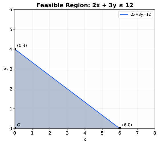
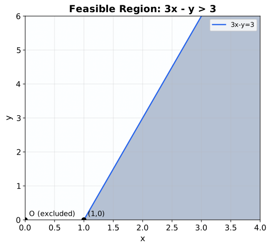
This chapter's own syllabus, and the underlying idea of a region bounded by straight-line limits, is not unique to any one board — the same linear-inequality graphing skill sits at the base of the business-mathematics and operations-research curriculum used across Indian commerce boards, precisely because at most / at least resource limits are a universal feature of managerial decision-making, not a peculiarity of any single syllabus.