Chemistry · Ch 1 — Solutions

Depression of Freezing Point

1.6.3

Depression of Freezing Point

At its freezing point, a substance has its solid and liquid phases in dynamic equilibrium. A useful way to state this: the freezing point is the temperature at which the vapour pressure of the substance in its liquid phase equals the vapour pressure in its solid phase.

Why the freezing point falls

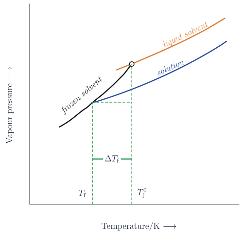
A solution freezes when its vapour pressure equals that of the pure solid solvent. Adding a non-volatile solute lowers the solvent's vapour pressure (Raoult's law), so the vapour-pressure curve of the solution sits below that of the pure solvent. The solution's lowered curve meets the solid-solvent curve only at a lower temperature. As a result, the freezing point of the solvent decreases.

Figure 1.8Diagram showing ΔTf, depression of the freezing point of a solvent in a solution.

Fig. 1.8 — Diagram showing ΔTf, depression of the freezing point of a solvent in a solution.

Drawn by us to help you understand the concept clearly, and verified to make sure it's accurate. For exams, practice from your textbook's own diagram.

What the Diagram Shows

The figure is a vapour pressure vs. temperature graph.

Y-axis: Vapour pressure of the solvent (in arbitrary units).
X-axis: Temperature (in Kelvin).

Three curves are plotted:

Frozen solvent curve – represents the vapour pressure of the pure solid solvent (ice, if the solvent is water).
Liquid solvent curve – shows how the vapour pressure of the pure liquid solvent changes with temperature.
Solution curve – lies below the liquid-solvent curve at every temperature, because adding a non-volatile solute lowers the vapour pressure of the solvent.

The liquid-solvent curve and the frozen-solvent curve intersect at a single point: $T_f^\circ$ , the freezing point of the pure solvent. At this temperature, solid and liquid solvent have the same vapour pressure.

The solution curve meets the frozen-solvent curve at a lower temperature, labelled $T_f$ . Dashed vertical lines drop from both intersection points to the x-axis. The horizontal distance between $T_f^\circ$ and $T_f$ on the x-axis is labelled $\Delta T_f$ — the depression of freezing point.

The Physical Idea

Freezing occurs when the vapour pressure of the liquid equals the vapour pressure of the solid.

For a pure solvent, this happens at $T_f^\circ$ .
When a non-volatile solute is added, the vapour pressure of the liquid decreases (Raoult’s law). The solid’s vapour pressure is unchanged.
Therefore, the liquid and solid vapour pressures now become equal at a lower temperature $T_f$ .

The depression $\Delta T_f = T_f^\circ - T_f$ is directly proportional to the molality ( $m$ ) of the solution:

\Delta T_f = K_f \cdot m

where

$K_f$ = molal freezing point depression constant (or cryoscopic constant) of the solvent, with units $\text{K kg mol}^{-1}$ .
$m$ = molality of the solute = $\dfrac{\text{moles of solute}}{\text{kg of solvent}}$ .

Key Formulas Derived from This Figure

If $w_2$ grams of solute (molar mass $M_2$ ) are dissolved in $w_1$ grams of solvent, the molality is:

m = \frac{w_2 / M_2}{w_1 / 1000} = \frac{1000 \, w_2}{M_2 \, w_1}

Substituting into $\Delta T_f = K_f m$ gives:

\Delta T_f = K_f \cdot \frac{1000 \, w_2}{M_2 \, w_1}

Rearranging to solve for the molar mass of the solute:

M_2 = \frac{K_f \cdot 1000 \, w_2}{\Delta T_f \cdot w_1}

The constant $K_f$ itself can be calculated from the solvent’s properties:

K_f = \frac{R \, M_1 \, (T_f^\circ)^2}{1000 \, \Delta_{\text{fus}} H}

where

$R$ = gas constant ( $8.314 \, \text{J mol}^{-1} \text{K}^{-1}$ )
$M_1$ = molar mass of the solvent (in $\text{g mol}^{-1}$ )
$T_f^\circ$ = freezing point of pure solvent (in K)
$\Delta_{\text{fus}} H$ = enthalpy of fusion of the solvent (in $\text{J g}^{-1}$ or $\text{J mol}^{-1}$ ).

--- …

Defining the depression

Let $T_f^{0}$ be the freezing point of the pure solvent and $T_f$ the freezing point after a non-volatile solute is dissolved in it. The depression of freezing point is

\Delta T_f = T_f^{0} - T_f

Proportional to molality

Just as with boiling-point elevation, for a dilute (ideal) solution the depression is directly proportional to the molality of the solute:

\Delta T_f \propto m

\Delta T_f = K_f\,m

Important

The proportionality constant $K_f$ is the Freezing Point Depression Constant or Molal Depression Constant (also called the cryoscopic constant). It depends on the nature of the solvent, and its unit is $\text{K kg mol}^{-1}$ . Values of $K_f$ for common solvents are listed in the accompanying constants table.

Building the molar-mass formula

For $w_2$ gram of solute of molar mass $M_2$ dissolved in $w_1$ gram of solvent, the molality is

m = \frac{w_2 / M_2}{w_1 / 1000}

Substituting into $\Delta T_f = K_f\,m$ :

\Delta T_f = \frac{K_f \times w_2 / M_2}{w_1 / 1000}

\Delta T_f = \frac{K_f \times w_2 \times 1000}{M_2 \times w_1}

Rearranging to make the molar mass the subject:

M_2 = \frac{K_f \times w_2 \times 1000}{\Delta T_f \times w_1}

So to determine $M_2$ , we need the masses $w_1$ and $w_2$ , the measured depression $\Delta T_f$ , and the molal freezing point depression constant of the solvent.

How $K_f$ and $K_b$ arise from solvent properties

The constants themselves can be related to fundamental properties of the solvent: …

Table 1.3Molal Boiling Point Elevation and Freezing Point Depression Constants for Some Solvents

Solvent	b. p./K	$K_b$ /K kg mol $^{-1}$	f. p./K	$K_f$ /K kg mol $^{-1}$
Water	373.15	0.52	273.0	1.86
Ethanol	351.5	1.20	155.7	1.99
Cyclohexane	353.74	2.79	279.55	20.00
Benzene	353.3	2.53	278.6	5.12
Chloroform	334.4	3.63	209.6	4.79
Carbon tetrachloride	350.0	5.03	250.5	31.8
Carbon disulphide	319.4	2.34	164.2	3.83

Start your 14-day free trial to unlock the full solution →

← Previous · 1.6.2Example 1.8 — The boiling point of benzene is 353.23 K. When 1.80 g of a non-volatil…Next · 1.6.3 →Example 1.9 — 45 g of ethylene glycol (C₂H₆O₂) is mixed with 600 g of water. Calcula…

Depression of Freezing Point