Physics · Ch 1 — Electric Charges and Fields

Continuous Charge Distribution

1.12

Continuous Charge Distribution

Why Continuous Charge Distributions?

Discrete point charges ( $q_1, q_2, \dots$ ) are mathematically simple, but real objects (like a charged metal sphere or a wire) contain an enormous number of microscopic charges. It is impractical to track each electron. Instead, we treat the charge as smeared out continuously over a line, surface, or volume — exactly as we treat a liquid's density without counting individual molecules.

This "macroscopic smoothing" ignores the microscopic granularity of charge but gives accurate results for distances much larger than the spacing between charges.

Three Types of Charge Density

For a small macroscopic element (large enough to contain many charges, but small on our scale), we define:

Linear charge density $\lambda$ (for a wire or thin rod):

\lambda = \frac{\Delta Q}{\Delta l}

$\Delta l$ = small length element, $\Delta Q$ = charge in it.
Unit: $\text{C/m}$ .

Surface charge density $\sigma$ (for a sheet or conductor surface):

\sigma = \frac{\Delta Q}{\Delta S}

$\Delta S$ = small area element, $\Delta Q$ = charge on it.
Unit: $\text{C/m}^2$ .

Volume charge density $\rho$ (for a 3D object):

\rho = \frac{\Delta Q}{\Delta V}

$\Delta V$ = small volume element, $\Delta Q$ = charge inside it.
Unit: $\text{C/m}^3$ .

These densities are functions of position — they can vary from point to point.

Electric Field from a Continuous Distribution

The strategy is the same as for discrete charges: Coulomb's law + superposition.

Pick an origin $O$ . Let $\mathbf{r}$ be the position vector of a point inside the charge distribution.
Consider a tiny volume element $\Delta V$ at $\mathbf{r}$ , carrying charge $\rho(\mathbf{r})\,\Delta V$ .
For a field point $P$ with position vector $\mathbf{R}$ , the distance from the charge element to $P$ is:

r' = |\mathbf{R} - \mathbf{r}|

and $\hat{\mathbf{r}}'$ is the unit vector pointing from the charge element to $P$ .

The electric field due to this single element is (Coulomb's law):

\Delta \mathbf{E} = \frac{1}{4\pi\varepsilon_0} \frac{\rho(\mathbf{r})\,\Delta V}{r'^{\,2}} \,\hat{\mathbf{r}}'

Superposition: total field is the sum over all volume elements: …

Figure 1.21Definition of linear, surface and volume charge densities. In each case, the element (Dl, DS, DV) chosen is small on the macroscopic scale but contains a very large number of microscopic constituents.

Fig. 1.21 — Definition of linear, surface and volume charge densities. In each case, the element (Dl, DS, DV) chosen is small on the macroscopic scale but contains a very large number of microscopic constituents.

Drawn by us to help you understand the concept clearly, and verified to make sure it's accurate. For exams, practice from your textbook's own diagram.

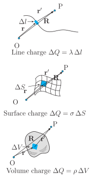
The figure presents three separate panels, each illustrating a different type of continuous charge distribution. In every panel, the same geometric setup is used: an origin O, a field point P, and three position vectors. The vector from O to a small charge element is labelled r, the vector from that element to P is labelled r′, and the vector from O directly to P is labelled R. This common structure emphasises that the electric field at P is always calculated by summing contributions from tiny charge elements, regardless of whether the charge is spread along a line, over a surface, or throughout a volume.

Top panel — Line charge distribution: A curved wire is shown, with a small segment of length $\Delta l$ highlighted. The charge on this segment is $\Delta Q = \lambda \, \Delta l$ , where $\lambda$ is the linear charge density (units: C/m). The wire is one-dimensional on the macroscopic scale, but $\Delta l$ is large enough to contain many microscopic charges.

Middle panel — Surface charge distribution: A curved, meshed sheet is depicted, with a small patch of area $\Delta S$ marked (the label $\Delta S$ is placed at the left side of the patch). The charge on this patch is $\Delta Q = \sigma \, \Delta S$ , where $\sigma$ is the surface charge density (units: C/m²). The sheet is two-dimensional macroscopically, but $\Delta S$ is microscopically large.

Bottom panel — Volume charge distribution: An irregular three-dimensional shape is shown, with a small volume element $\Delta V$ inside it. The charge in this element is $\Delta Q = \rho \, \Delta V$ , where $\rho$ is the volume charge density (units: C/m³). The volume is three-dimensional, and $\Delta V$ is macroscopically small but contains a huge number of charges.

The physical idea is that for a continuous distribution, we replace the discrete sum over point charges with an integral over infinitesimal charge elements. The textbook uses this figure to derive the electric field at point P due to a volume charge distribution. Starting from Coulomb’s law for a single element:

\Delta \mathbf{E} = \frac{1}{4\pi\varepsilon_0} \frac{\rho \, \Delta V}{r'^2} \, \hat{\mathbf{r}}'

where $r'$ is the distance from the element to P and $\hat{\mathbf{r}}'$ is the unit vector pointing from the element to P. Summing over all elements gives the total field: …

Start your 14-day free trial to unlock the full solution →

← Previous · 1.11Dipole in a Uniform External Field Next · 1.13 →Gauss's Law