Mathematics · Ch 12 — Application of Definite Integration

Area between two curves

12.1.2

Area between two curves

This is the chapter's longest section: it extends the single-curve idea of 5.1.1 to two curves at once, works out what happens when a curve dips below the X-axis or changes sign partway through an interval, and then runs through fourteen further solved examples that between them cover every technique the exercises need -- straight lines, parabolas in both orientations, the ellipse, two intersecting parabolas, a curve-and-line region, and a circular sector.

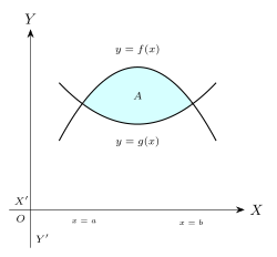
Area between two curves (Fig. 5.5). Let $y = f(x)$ and $y = g(x)$ be two curves that cross each other, enclosing a lens-shaped region $A$ between $x = a$ and $x = b$ (their points of intersection). If $A_1$ is the area between $y = f(x)$ , the X-axis, and the lines $x = a, x = b$ , and $A_2$ is the corresponding area for $y = g(x)$ , then the area actually enclosed between the two curves is the difference of these two areas, taken positive:

A = |A_1 - A_2|, \qquad A = \left|\int_a^b f(x)\,dx - \int_a^b g(x)\,dx\right|

Figure 5.5Fig. 5.5 -- lens-shaped region between two intersecting curves

$Fig. 5.5 — Fig. 5.5 -- lens-shaped region between two intersecting curves$

Drawn by us to help you understand the concept clearly, and verified to make sure it's accurate. For exams, practice from your textbook's own diagram.

What this figure shows. This figure sets up the area-between-two-curves formula. It shows two curves y = f(x) (the upper one) and y = g(x) (the lower one) crossing each other at two points, so that between the vertical lines x = a and x = b they enclose a lens-shaped shaded region A between them, without the X-axis playing any part in the boundary. The picture is the geometric justification for defining this area as the absolute difference of the two curves' separate areas under the X-axis, A1 (for f) minus A2 (for g), between t …

The points of intersection $x = a, x = b$ are found first, by solving the two equations simultaneously -- they are not given directly in the problem, they have to be worked out, and this step is where most of the algebra in this section's examples happens.

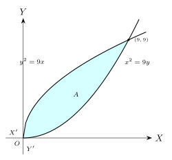
Solved Example -- $y^2 = 9x$ and $x^2 = 9y$ (Fig. 5.6). Squaring the second equation and substituting the first, $x^4 = 81y^2 = 81(9x) = 729x$ , so $x(x^3 - 9^3) = 0$ , giving $x = 0$ or $x = 9$ , and correspondingly $y = 0$ or $y = 9$ . The curves meet at $(0,0)$ and $(9,9)$ . Between these, the rightward parabola $y = \sqrt{9x}$ lies above the upward parabola $y = x^2/9$ , so

A = \int_0^9 \sqrt{9x}\,dx - \int_0^9 \frac{x^2}{9}\,dx = \left[2x^{3/2}\right]_0^9 - \left[\frac{x^3}{27}\right]_0^9 = 54 - 27 = 27 \text{ sq. units}

Figure 5.6Fig. 5.6 -- region between y^2 = 9x and x^2 = 9y (Solved Example)

$Fig. 5.6 — Fig. 5.6 -- region between y^2 = 9x and x^2 = 9y (Solved Example)$

Drawn by us to help you understand the concept clearly, and verified to make sure it's accurate. For exams, practice from your textbook's own diagram.

What this figure shows. This figure accompanies the example that finds the area enclosed between the two parabolas y^2 = 9x (opening rightwards, sagging below the X-axis in the picture) and x^2 = 9y (opening upwards). It shows both curves passing through the origin O and meeting again at a labelled point P(a, a), with the thin sliver-shaped region OBP between the two arcs, near the origin, hatched. The picture confirms that the two curves cross exactly twice, at O and at (9, 9), and that the enclosed region lies entirely in the first quadrant between these …

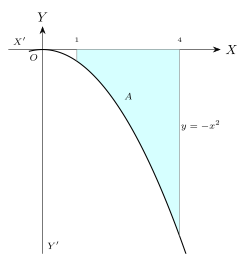
What if the curve dips below the X-axis? If $f(x) \le 0$ throughout $[a, b]$ , the raw integral $\int_a^b f(x)\,dx$ comes out negative (Fig. 5.7), because every strip's signed height is negative -- but an area can never be negative, so the actual area is the absolute value $\left|\int_a^b f(x)\,dx\right|$ . More generally, whether the curve is above or below the axis throughout the interval, the enclosed area is $\left|\int_a^b f(x)\,dx\right|$ .

Solved Example -- $y = -x^2$ between $x=1$ and $x=4$ (Fig. 5.7). $\displaystyle\int_1^4 (-x^2)\,dx = \left[-\frac{x^3}{3}\right]_1^4 = -\frac{64}{3} + \frac{1}{3} = -21$ . Taking the absolute value, the area is $21$ square units.

Figure 5.7Fig. 5.7 -- region under the negative curve y = -x^2 (Solved Example)

$Fig. 5.7 — Fig. 5.7 -- region under the negative curve y = -x^2 (Solved Example)$

Drawn by us to help you understand the concept clearly, and verified to make sure it's accurate. For exams, practice from your textbook's own diagram.

What this figure shows. This figure illustrates the case where the bounding curve dips below the X-axis. It draws the downward parabola y = -x^2, opening below the X-axis, together with the two vertical lines x = 1 and x = 4, and fills the region trapped between the curve and the X-axis over that interval with vertical strips. Because the whole shaded region lies below the X-axis, the figure is the visual reminder that the raw definite integral over this interval comes out negative and that the actual area is its a …

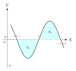
What if the curve changes sign inside the interval (Fig. 5.8)? If $f(x) \le 0$ on part of $[a, b]$ (say from $a$ to an interior crossing point $t$ ) and $f(x) \ge 0$ on the rest (from $t$ to $b$ ), the two pieces $A_1$ and $A_2$ must be found and made positive separately, then added -- a single integral over the whole interval would let the negative and positive parts cancel and understate the true area:

A = A_1 + A_2 = \left|\int_a^t f(x)\,dx\right| + \left|\int_t^b f(x)\,dx\right|

Figure 5.8Fig. 5.8 -- a curve with regions on both sides of the X-axis

$Fig. 5.8 — Fig. 5.8 -- a curve with regions on both sides of the X-axis$

Drawn by us to help you understand the concept clearly, and verified to make sure it's accurate. For exams, practice from your textbook's own diagram.

What this figure shows. This figure shows a general curve that dips below the X-axis on the left part of an interval [a, b] and rises above it on the right part, crossing the X-axis at an interior point marked t. The lower part of the region, from x = a to x = t, is labelled A1 and lies below the axis; the upper part, from x = t to x = b, is labelled A2 and lies above the axis. The figure is the template for the rule that the total unsigned area equals the absolute value of the integral over A1 plus the absolute value of the integral over A2, added separately rather than as one signe …

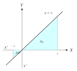
Solved Example -- $y = x$ between $x=-1$ and $x=4$ (Fig. 5.9). The line crosses the X-axis at the origin, which splits the interval. For $-1 \le x \le 0$ : $A_1 = \int_{-1}^0 x\,dx = \left[\frac{x^2}{2}\right]_{-1}^0 = -\frac{1}{2}$ , so $|A_1| = \frac{1}{2}$ . For $0 \le x \le 4$ : $A_2 = \int_0^4 x\,dx = \frac{16}{2} = 8$ . Adding, the required area is $\frac{1}{2} + 8 = \frac{17}{2}$ square units.

Figure 5.9Fig. 5.9 -- region under the line y = x split at the origin (Solved Example)

$Fig. 5.9 — Fig. 5.9 -- region under the line y = x split at the origin (Solved Example)$

Drawn by us to help you understand the concept clearly, and verified to make sure it's accurate. For exams, practice from your textbook's own diagram.

What this figure shows. This figure accompanies the example that finds the area bounded by the straight line y = x, the X-axis, and the two vertical lines x = -1 and x = 4. It draws the line through the origin at 45 degrees, marks the boundary lines x = -1 and x = 4, and hatches the two triangular regions separately: a small one below the X-axis between x = -1 and x = 0 (labelled implicitly as the region A1 in the solution) and a larger one above the X-axis between x = 0 and x = 4 (region A2), showing visually why the line's own zero at the origin is exactly the split point used …

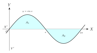
Solved Example -- $y = \sin x$ from $0$ to $2\pi$ (Fig. 5.10). Since $\sin x \ge 0$ on $[0, \pi]$ and $\sin x \le 0$ on $[\pi, 2\pi]$ , the two humps are found separately. $A_1 = \int_0^\pi \sin x\,dx = [-\cos x]_0^\pi = -(-1) - (-1) = 2$ . $A_2 = \int_\pi^{2\pi} \sin x\,dx = [-\cos x]_\pi^{2\pi} = -1 - 1 = -2$ , so $|A_2| = 2$ . Total area $= 2 + 2 = 4$ square units.

Figure 5.10Fig. 5.10 -- one full period of y = sin x from 0 to 2 pi (Solved Example)

$Fig. 5.10 — Fig. 5.10 -- one full period of y = sin x from 0 to 2 pi (Solved Example)$

Drawn by us to help you understand the concept clearly, and verified to make sure it's accurate. For exams, practice from your textbook's own diagram.

What this figure shows. This figure shows one complete wave of the sine curve y = sin x drawn from x = 0 to x = 2 pi, with the hump lying above the X-axis between 0 and pi hatched and labelled A1 and the trough lying below the X-axis between pi and 2 pi hatched and labelled A2. It illustrates why finding the total enclosed area needs two separate integrals of equal magnitude but opposite sign, one for each hump, whose absolute values are then added together rather than allowed to canc …

Two further problems (worked in the question bank as the chapter's Activity, since the book leaves them for the student to complete): finding the same total-unsigned-area for $y = \sin x$ over the longer interval $0$ to $4\pi$ (which repeats the same $\pi$ -by- $\pi$ splitting four times), and for $y = \cos x$ over the three interval choices $0$ to $\pi/2$ , $\pi/2$ to $\pi$ , and $0$ to $\pi$ (where $\cos x$ is positive on the first sub-interval and negative on the second, so the third case again needs the two pieces added).

A second bank of solved examples now works through the remaining standard shapes.

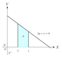
Ex. -- line $2y + x = 8$ between $x=2$ and $x=4$ (Fig. 5.11). Rewriting the line as $y = \frac{1}{2}(8-x)$ and integrating, $A = \int_2^4 \frac{1}{2}(8-x)\,dx = \frac{1}{2}\left[8x - \frac{x^2}{2}\right]_2^4 = 5$ square units.

Figure 5.11Fig. 5.11 -- trapezium under the line 2y + x = 8 (Solved Example)

$Fig. 5.11 — Fig. 5.11 -- trapezium under the line 2y + x = 8 (Solved Example)$

Drawn by us to help you understand the concept clearly, and verified to make sure it's accurate. For exams, practice from your textbook's own diagram.

What this figure shows. This figure, opening the chapter's second bank of solved examples, shows the straight line 2y + x = 8 sloping downward through the first quadrant, together with the two vertical lines x = 2 and x = 4, with the trapezium-shaped region between the line, the X-axis, and these two verticals hatched. It is the picture for the example that rewrites the line as y = (1/2)(8 - x) before integrating it between x = 2 and x = 4 to get the trapezium' …

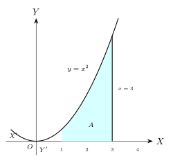
Ex. -- three curve-and-axis regions. (i) For $y = x^2$ between $x=1$ and $x=3$ (Fig. 5.12), $A = \int_1^3 x^2\,dx = \left[\frac{x^3}{3}\right]_1^3 = \frac{26}{3}$ sq. units.

Figure 5.12Fig. 5.12 -- region under y = x^2 up to x = 3 (second worked example)

$Fig. 5.12 — Fig. 5.12 -- region under y = x^2 up to x = 3 (second worked example)$

Drawn by us to help you understand the concept clearly, and verified to make sure it's accurate. For exams, practice from your textbook's own diagram.

What this figure shows. This figure accompanies the first part of a three-part worked example on areas bounded by a curve, the X-axis and given lines. It draws the parabola y = x^2 and hatches the region under the rising arc between x = 1 and the marked line x = 3, showing the vertical-strip region whose integral is evaluated to give the area for this part of the example. …

(ii) For $y^2 = 4x$ (upper branch $y = 2\sqrt x$ ) between $x=1$ and $x=4$ (Fig. 5.13), $A = \int_1^4 2\sqrt x\,dx = \left[\frac{4}{3}x^{3/2}\right]_1^4 = \frac{28}{3}$ sq. units.

Figure 5.13Fig. 5.13 -- region under y^2 = 4x between x = 1 and x = 4 (second worked example, part ii)

$Fig. 5.13 — Fig. 5.13 -- region under y^2 = 4x between x = 1 and x = 4 (second worked example, part ii)$

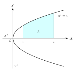
Drawn by us to help you understand the concept clearly, and verified to make sure it's accurate. For exams, practice from your textbook's own diagram.

What this figure shows. This figure illustrates the second part of the three-part worked example, showing the rightward-opening parabola y^2 = 4x with its upper branch drawn, and the region between the curve, the X-axis, and the two vertical lines x = 1 and x = 4 hatched with a rectangular grid pattern. It is the picture for integrating the upper-branch function y = 2 times the square root of x between x = 1 and x = 4. …

(iii) For $y = \sin x$ between $x=-\pi/2$ and $x=\pi/2$ (Fig. 5.14), the curve is negative on the left half and positive on the right half, so the two halves are found separately and added, each contributing $1$ , giving a total of $2$ sq. units.

Figure 5.14Fig. 5.14 -- region under y = sin x from x = -pi/2 to x = pi/2 (second worked example, part iii)

$Fig. 5.14 — Fig. 5.14 -- region under y = sin x from x = -pi/2 to x = pi/2 (second worked example, part iii)$

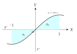
Drawn by us to help you understand the concept clearly, and verified to make sure it's accurate. For exams, practice from your textbook's own diagram.

What this figure shows. This figure illustrates the third part of the three-part worked example. It shows the sine curve drawn from x = -pi/2 to x = pi/2, with the small trough below the X-axis on the left of the origin and the matching hump above the X-axis on the right, both hatched, showing that although the curve is symmetric about the origin, the areas on the two sides must still be found and added as separate unsigned pieces rather than as one signed integral, since one lies below the axis and the other above it. …

Ex. -- parabola $y^2 = 16x$ and its latus rectum $x=4$ (Fig. 5.15). By symmetry about the X-axis, the total area is twice the area of just the upper half: $A = 2\int_0^4 4\sqrt x\,dx = 2\left[\frac{8}{3}x^{3/2}\right]_0^4 = \frac{128}{3}$ sq. units.

Figure 5.15Fig. 5.15 -- region bounded by the parabola y^2 = 16x and its latus rectum x = 4 (Solved Example)

$Fig. 5.15 — Fig. 5.15 -- region bounded by the parabola y^2 = 16x and its latus rectum x = 4 (Solved Example)$

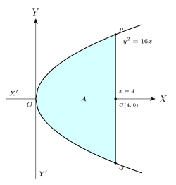
Drawn by us to help you understand the concept clearly, and verified to make sure it's accurate. For exams, practice from your textbook's own diagram.

What this figure shows. This figure accompanies the example that finds the area of the region bounded by the parabola y^2 = 16x and the vertical line x = 4 (its latus rectum). It draws the parabola opening rightwards from the origin O, marks the point C(4, 0) on the X-axis where the latus rectum crosses it, and hatches the full bow-shaped region POQ bounded by the two symmetric branches P and Q of the parabola and the line x = 4, showing why the calculation doubles the area of just the upper half POC before doubling it for the full symmetric region. …

Ex. -- $x^2 = 16y$ between $y=1$ and $y=4$ (Fig. 5.16). Here it is natural to integrate with respect to $y$ : $x = 4\sqrt y$ , so $A = \int_1^4 4\sqrt y\,dy = \left[\frac{8}{3}y^{3/2}\right]_1^4 = \frac{56}{3}$ sq. units.

Figure 5.16Fig. 5.16 -- region bounded by x^2 = 16y between y = 1 and y = 4 (Solved Example)

$Fig. 5.16 — Fig. 5.16 -- region bounded by x^2 = 16y between y = 1 and y = 4 (Solved Example)$

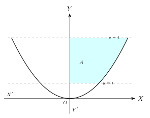
Drawn by us to help you understand the concept clearly, and verified to make sure it's accurate. For exams, practice from your textbook's own diagram.

What this figure shows. This figure accompanies the example that finds the area of the region between the upward parabola x^2 = 16y, the Y-axis, and the two horizontal lines y = 1 and y = 4, lying in the first quadrant. It shows the parabola's arc together with the two horizontal boundary lines labelled y = 1 and y = 4, with the strip of the region between them, up to the curve, filled with horizontal hatching -- the picture that motivates integrating with respect to y rather than x for this particular region. …

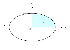
Ex. -- area of the ellipse $\frac{x^2}{a^2}+\frac{y^2}{b^2}=1$ (Fig. 5.17). By the ellipse's symmetry about both axes, the total area is four times the area of the first-quadrant quarter alone. Solving the equation for $y$ gives $y = \frac{b}{a}\sqrt{a^2 - x^2}$ for $y>0$ , so $A = 4\int_0^a \frac{b}{a}\sqrt{a^2-x^2}\,dx$ . Using the standard integral of $\sqrt{a^2-x^2}$ and evaluating between $0$ and $a$ , everything collapses to $A = \pi a b$ square units

Figure 5.17Fig. 5.17 -- one quadrant of the ellipse x^2/a^2 + y^2/b^2 = 1 (Solved Example)

$Fig. 5.17 — Fig. 5.17 -- one quadrant of the ellipse x^2/a^2 + y^2/b^2 = 1 (Solved Example)$

Drawn by us to help you understand the concept clearly, and verified to make sure it's accurate. For exams, practice from your textbook's own diagram.

What this figure shows. This figure accompanies the example that derives the well-known formula for the area of an ellipse. It draws the full ellipse with semi-axes a and b, marks the points Q(0, b) on the Y-axis and P(a, 0) on the X-axis, and hatches only the quarter of the ellipse lying in the first quadrant, between O, P and Q. The picture is the basis for the argument that, by the symmetry of the ellipse about both axes, the total area is exactly four times this single hatched quarter. …

-- the familiar formula for the area of an ellipse, derived here purely from integration rather than quoted.

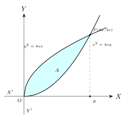
Ex. -- region between $y^2 = 4ax$ and $x^2 = 4ay$ , for $a>0$ (Fig. 5.18). Exactly the same substitution technique as the $y^2=9x$ , $x^2=9y$ example above, but now with a general parameter $a$ : the curves meet at $(0,0)$ and $(4a, 4a)$ , and subtracting the area under one parabola from the area under the other over $[0, 4a]$ gives $A = \frac{16}{3}a^2$ square units.

Figure 5.18Fig. 5.18 -- region between the parabolas y^2 = 4ax and x^2 = 4ay (Solved Example)

$Fig. 5.18 — Fig. 5.18 -- region between the parabolas y^2 = 4ax and x^2 = 4ay (Solved Example)$

Drawn by us to help you understand the concept clearly, and verified to make sure it's accurate. For exams, practice from your textbook's own diagram.

What this figure shows. This figure accompanies the example that finds the area lying between the two parabolas y^2 = 4ax (opening rightwards, sagging below the axis in the drawing) and x^2 = 4ay (opening upwards). It shows both curves starting at the origin O and meeting again at a labelled point P(4a, 4a), with the point B marked on the X-axis directly below P, and the thin curved sliver of region between the two arcs, close to the origin, hatched -- the same general shape as Fig. 5.6 but now for the general parameter a rather than the fixed numbers 9 …

…

Figure 5.19Fig. 5.19 -- region between the parabola y = x^2 and the line y = 4 (Solved Example)

$Fig. 5.19 — Fig. 5.19 -- region between the parabola y = x^2 and the line y = 4 (Solved Example)$

Drawn by us to help you understand the concept clearly, and verified to make sure it's accurate. For exams, practice from your textbook's own diagram.

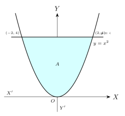
What this figure shows. This figure accompanies the example that finds the area bounded by the upward parabola y = x^2 and the horizontal line y = 4. It draws the parabola's arc rising steeply on both sides of the Y-axis up to where it meets the horizontal line y = 4, and fills the entire cup-shaped region between the parabola and the line with dense horizontal hatching, showing the symmetric region whose area the example finds by doubling the area of just its right half, computed as an integral with respect to y. …

Figure 5.20Fig. 5.20 -- circular sector cut by y = x from the circle x^2 + y^2 = 16 (Solved Example)

$Fig. 5.20 — Fig. 5.20 -- circular sector cut by y = x from the circle x^2 + y^2 = 16 (Solved Example)$

Drawn by us to help you understand the concept clearly, and verified to make sure it's accurate. For exams, practice from your textbook's own diagram.

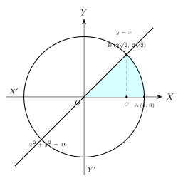
What this figure shows. This figure accompanies the final worked example of the section, which finds the area of the sector cut off in the first quadrant by the circle x^2 + y^2 = 16 and the line y = x. It draws the circle together with the 45-degree line y = x through the origin, marks their intersection point B(2 root 2, 2 root 2) and the point A(4, 0) where the circle meets the X-axis, marks the foot C of the perpendicular from B onto the X-axis, and hatches the pie-slice sector OCB A bounded by the line, the arc, and the X-axis -- the picture behind splitting the area into a triangular piece under the line and a curved piece under th …

Start your 14-day free trial to unlock the full solution →

← Previous · 12.1.1Area under a curve Next →Q1 — Find the area bounded by the curve y² = 4ax, X-axis and the lines x = …