Mathematics · Ch 12 — Application of Definite Integration

Area under the curve

The previous chapter defined the definite integral $\int_a^b f(x)\,dx$ as the limit of a sum, and proved the Fundamental Theorem of Integral Calculus: if $\int f(x)\,dx = \phi(x)$ , then $\int_a^b f(x)\,dx = \phi(b) - \phi(a)$ . This chapter's whole purpose is to read that same number geometrically -- as an area -- and to use it to measure the plane regions trapped by curves that appear in Class 12 mathematics: parabolas, circles, ellipses, straight lines, and trigonometric curves.

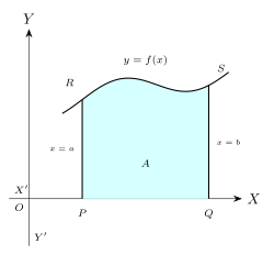
The geometric idea (Fig. 5.1) is this. Suppose a curve $y = f(x)$ is continuous on an interval $[a, b]$ and stays on or above the X-axis there, i.e. $f(x) \ge 0$ for every $x$ in $[a, b]$ . Draw the two vertical lines $x = a$ and $x = b$ . These two lines, together with the curve above and the X-axis below, close off a bounded region -- call its area $A$ . If this region is sliced into a very large number of extremely thin vertical strips, each strip is (to a very good approximation) a rectangle of height $y = f(x)$ and width $dx$ , so its area is $y\,dx$ . Adding up all these strip-areas from $x = a$ to $x = b$ is exactly what the definite integral does, so:

A = \int_a^b f(x)\,dx = \int_{x=a}^{x=b} y\,dx

Figure 5.1Fig. 5.1 -- area under y = f(x) as a definite integral

$Fig. 5.1 — Fig. 5.1 -- area under y = f(x) as a definite integral$

Drawn by us to help you understand the concept clearly, and verified to make sure it's accurate. For exams, practice from your textbook's own diagram.

What this figure shows. This opening figure recalls the geometric meaning of a definite integral carried over from the previous chapter. It draws a curve y = f(x) rising above the X-axis between two vertical lines x = a and x = b, with the region R S Q P between the curve, the X-axis, and these two lines shaded with horizontal strips. The labelled shaded region is called A, and the figure is the visual anchor for the statement that A equals the definite integral of f(x) from a to b, i.e. that the Fundamental Theorem of Integral Calculus converts a geometric area into a difference of antiderivative values, phi(b) minus phi(a).

5.1: Fig. 5.1 -- area under y = f(x) as a definite integral.

Before this idea can be applied to a specific problem, two practical skills matter as much as the formula itself: knowing the shape of the curve involved (is it a parabola, an ellipse, a line, a sine wave?) and being able to sketch it, at least roughly, so that the correct bounded region -- and not some other region enclosed by the same equations -- is the one being measured. The rest of the chapter builds on this single idea in two directions: finding the area under one curve alone (Section 5.1.1), and finding the area enclosed between two curves that cross each other (Section 5.1.2).

← Previous chapterCh 11 — Definite Integration Next · 12.1.1 →Area under a curve