Mathematics · Ch 12 — Application of Definite Integration

Area under a curve

12.1.1

Area under a curve

This section states, side by side, the two basic forms the area formula can take, and then works through the chapter's first complete example.

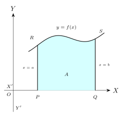
1. Area with the X-axis as one boundary (Fig. 5.2). If a curve $y = f(x)$ is continuous on $[a, b]$ with $f(x) \ge 0$ throughout, the area $A$ of the region bounded by the curve, the X-axis, and the two vertical lines $x = a$ , $x = b$ is

A = \int_{x=a}^{x=b} y\,dx = \int_a^b f(x)\,dx

Here the strips used to build up the area are vertical: each one runs from the X-axis up to the curve, has width $dx$ , and height $y$ .

Figure 5.2Fig. 5.2 -- vertical-strip area bounded by y = f(x), the X-axis and x = a, x = b

$Fig. 5.2 — Fig. 5.2 -- vertical-strip area bounded by y = f(x), the X-axis and x = a, x = b$

Drawn by us to help you understand the concept clearly, and verified to make sure it's accurate. For exams, practice from your textbook's own diagram.

What this figure shows. This figure is the working picture for the first area formula. It shows a curve y = f(x) with the region PQSR between the curve, the X-axis, and the two vertical lines x = a and x = b filled with closely spaced vertical strips labelled A, with P and Q marking where the boundary lines x = a and x = b meet the X-axis. It is the standard picture used whenever the area is computed by integrating with respect to x, i.e. by summing thin vertical strips of height y = f(x) and width dx from x = a to x …

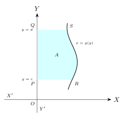
2. Area with the Y-axis as one boundary (Fig. 5.3). Sometimes it is more natural to describe a curve as $x = g(y)$ , expressing $x$ as a function of $y$ -- for instance a sideways-opening parabola, or any curve where slicing horizontally gives simpler strips than slicing vertically. In that case, the area bounded by the curve, the Y-axis, and the two horizontal lines $y = c$ , $y = d$ is found by summing horizontal strips of width $x = g(y)$ and height $dy$ , running from $y = c$ up to $y = d$ :

A = \int_{y=c}^{y=d} x\,dy = \int_{y=c}^{y=d} g(y)\,dy

Figure 5.3Fig. 5.3 -- horizontal-strip area bounded by x = g(y), the Y-axis and y = c, y = d

$Fig. 5.3 — Fig. 5.3 -- horizontal-strip area bounded by x = g(y), the Y-axis and y = c, y = d$

Drawn by us to help you understand the concept clearly, and verified to make sure it's accurate. For exams, practice from your textbook's own diagram.

What this figure shows. This is the Y-axis counterpart of Fig. 5.2. It shows a curve x = g(y) together with the region PQSR bounded by the curve, the Y-axis, and the two horizontal lines y = c and y = d, filled with closely spaced horizontal strips and labelled A, with P and Q marking where the lines y = c and y = d meet the Y-axis and S, R marking where they meet the curve. It is the picture used whenever it is easier to treat x as a function of y and integrate with respect to y instead of x, summing thin horizontal strips of width x = g(y) and height dy from y = c …

Deciding which of these two forms to use for a given problem is mostly a matter of which variable the curve's equation is more naturally solved for, and which choice keeps the same curve as the boundary throughout the strip (rather than switching between two different branches partway through).

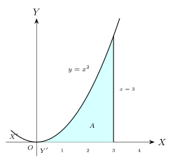
Solved Example -- Area under $y = x^2$ up to $x = 3$ (Fig. 5.4). Find the area bounded by the curve $y = x^2$ , the Y-axis, the X-axis, and the line $x = 3$ . Since the parabola lies on or above the X-axis for every $x \ge 0$ , formula 1 applies directly with $a = 0$ and $b = 3$ : …

Figure 5.4Fig. 5.4 -- region under y = x^2 up to x = 3 (Solved Example)

$Fig. 5.4 — Fig. 5.4 -- region under y = x^2 up to x = 3 (Solved Example)$

Drawn by us to help you understand the concept clearly, and verified to make sure it's accurate. For exams, practice from your textbook's own diagram.

What this figure shows. This figure illustrates the chapter's first fully worked example. It draws the parabola y = x^2 opening upward from the origin, together with the vertical line x = 3, and shades the region bounded by the parabola, the Y-axis, the X-axis and the line x = 3 with diagonal hatching. The picture makes clear that the shaded region is a single vertical strip region running from x = 0 to x = 3, directly under the rising arc of the parabola, which is exactly the region the accompanying solved example integrates to get a …

Start your 14-day free trial to unlock the full solution →

← Previous · introArea under the curve Next · 12.1.2 →Area between two curves