Mathematics · Ch 14 — Probability Distributions
Cumulative Distribution Functions (c. d. f.)
Cumulative Distribution Functions (c. d. f.)
The cumulative distribution function of a continuous random variable extends the discrete definition in the natural way, replacing the sum by an integral. If is a continuous random variable with p.d.f. on , its c.d.f. is for . While a discrete c.d.f. is a step function, a continuous c.d.f. is always a non-decreasing continuous function.
Worked examples.
Example 3. For , (Example 1 of section 7.4.1), find .
.
Example 4. For , , find .
.
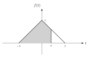
Example 5. has p.d.f. for and for . Find the c.d.f. .
The density is defined piecewise, so is built piecewise too. For : ; in particular . For : . Collecting every piece: for ; for ; for ; for . The way accumulates is illustrated in Fig. 7.1, which shows the triangular density itself: is the area under this triangle from up to (the shaded region), growing from at , reaching exactly at (half of the triangle's total area of ), and climbing to at once the whole triangle is covered — matching the piecewise formula just derived. …
Drawn by us to help you understand the concept clearly, and verified to make sure it's accurate. For exams, practice from your textbook's own diagram.
What this figure shows. Fig. 7.1 sketches the graph of the piecewise cumulative distribution function derived in the worked example beside it, for a density that rises linearly on (-1, 0) and falls linearly on (0, 1): the c.d.f. is 0 for x <= -1, climbs along the curve (x+1)^2/2 for -1 < x <= 0 reaching 1/2 at x = 0, then continues along 1/2 + x - x^2/2 for 0 < x < 1 up to 1, and stays flat at 1 for x >= 1 — a single continuous, non-decreasing curve from 0 to 1 with no jumps, unlike a …