Physics · Ch 5 — Work, Energy and Power

The Scalar Product

5.1.1

The Scalar Product

The Scalar Product of Two Vectors

Vectors can be multiplied in two fundamentally different ways. One way produces a scalar quantity — this is the scalar product (also called the dot product). The other way produces a new vector — the vector product (or cross product), which you will study in Chapter 6.

The scalar product of two vectors $\mathbf{A}$ and $\mathbf{B}$ is written as $\mathbf{A} \cdot \mathbf{B}$ (read as "A dot B"). The dot in the notation is the reason it is also called the dot product.

Definition of the Scalar Product

The scalar product of two vectors $\mathbf{A}$ and $\mathbf{B}$ is defined as the product of their magnitudes and the cosine of the angle $\theta$ between them:

\mathbf{A} \cdot \mathbf{B} = |\mathbf{A}| \, |\mathbf{B}| \cos \theta = AB \cos \theta

where $A = |\mathbf{A}|$ , $B = |\mathbf{B}|$ , and $\theta$ is the smaller angle between $\mathbf{A}$ and $\mathbf{B}$ when they are placed tail-to-tail, with $0 \le \theta \le \pi$ .

Important

The result of a scalar product is always a scalar (a real number), never a vector. It can be positive, negative, or zero, depending on the angle $\theta$ .

Geometric Meaning

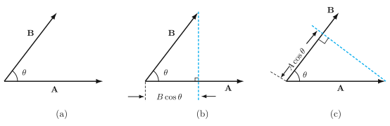
The scalar product has a clear geometric interpretation. It equals the product of the magnitude of one vector and the projection of the other vector onto it.

$A \cos \theta$ is the component (projection) of $\mathbf{A}$ along the direction of $\mathbf{B}$ .
$B \cos \theta$ is the component (projection) of $\mathbf{B}$ along the direction of $\mathbf{A}$ .

So $\mathbf{A} \cdot \mathbf{B} = A (B \cos \theta) = B (A \cos \theta)$ .

Tip

When you need the component of a vector $\mathbf{A}$ along a direction given by a unit vector $\hat{\mathbf{n}}$ , simply take the dot product: $\mathbf{A} \cdot \hat{\mathbf{n}} = A \cos \theta$ .

Properties of the Scalar Product

The scalar product obeys several important properties. Each one is derived directly from the definition.

›Proof

Property 1: Commutative Law

The scalar product is commutative: $\mathbf{A} \cdot \mathbf{B} = \mathbf{B} \cdot \mathbf{A}$ .

From the definition:

$\mathbf{A} \cdot \mathbf{B} = AB \cos \theta$

$\mathbf{B} \cdot \mathbf{A} = BA \cos \theta$

Since $AB = BA$ (ordinary multiplication of magnitudes is commutative) and $\cos \theta$ is the same in both cases, the two expressions are equal.

›Proof

Property 2: Distributive Law

The scalar product is distributive over vector addition: $\mathbf{A} \cdot (\mathbf{B} + \mathbf{C}) = \mathbf{A} \cdot \mathbf{B} + \mathbf{A} \cdot \mathbf{C}$ .

This property can be understood geometrically. Consider the projection of $\mathbf{B} + \mathbf{C}$ onto $\mathbf{A}$ . The projection of the sum equals the sum of the individual projections. Multiplying each projection by $A$ gives the result. A full algebraic proof using components is straightforward and will be shown after we introduce the component form.

›Proof

Property 3: Scalar Multiplication

For any scalar $\lambda$ :

$(\lambda \mathbf{A}) \cdot \mathbf{B} = \lambda (\mathbf{A} \cdot \mathbf{B}) = \mathbf{A} \cdot (\lambda \mathbf{B})$

Proof: $(\lambda \mathbf{A}) \cdot \mathbf{B} = |\lambda \mathbf{A}| B \cos \theta = |\lambda| A B \cos \theta$ (taking the sign of $\lambda$ into account through the magnitude). More precisely, if $\lambda > 0$ , the direction of $\lambda \mathbf{A}$ is the same as $\mathbf{A}$ , so $(\lambda \mathbf{A}) \cdot \mathbf{B} = \lambda A B \cos \theta = \lambda (\mathbf{A} \cdot \mathbf{B})$ . If $\lambda < 0$ , the direction reverses, and $\cos \theta$ changes sign accordingly, but the equality still holds. The same reasoning applies to $\mathbf{A} \cdot (\lambda \mathbf{B})$ .

›Proof

Property 4: Dot Product with Itself

The scalar product of a vector with itself equals the square of its magnitude:

$\mathbf{A} \cdot \mathbf{A} = A^2$

When $\mathbf{A}$ is dotted with itself, the angle between them is $\theta = 0$ . Since $\cos 0 = 1$ , we get $\mathbf{A} \cdot \mathbf{A} = A \cdot A \cdot 1 = A^2$ .

›Proof

Property 5: Orthogonal Vectors

Two non-zero vectors $\mathbf{A}$ and $\mathbf{B}$ are perpendicular (orthogonal) if and only if their scalar product is zero:

$\mathbf{A} \cdot \mathbf{B} = 0 \iff \mathbf{A} \perp \mathbf{B}$

If $\mathbf{A} \perp \mathbf{B}$ , then $\theta = 90^\circ$ and $\cos 90^\circ = 0$ , so $\mathbf{A} \cdot \mathbf{B} = AB(0) = 0$ . Conversely, if $\mathbf{A} \cdot \mathbf{B} = 0$ and neither $A$ nor $B$ is zero, then $\cos \theta = 0$ , which means $\theta = 90^\circ$ (or $270^\circ$ , but the angle between vectors is taken as the smaller one, $0 \le \theta \le \pi$ ).

Scalar Product in Component Form

Any vector can be expressed in terms of its components along the coordinate axes using unit vectors. In three dimensions, using the right-handed Cartesian coordinate system with unit vectors $\hat{\mathbf{i}}$ , $\hat{\mathbf{j}}$ , $\hat{\mathbf{k}}$ along the $x$ , $y$ , $z$ axes respectively:

\mathbf{A} = A_x \hat{\mathbf{i}} + A_y \hat{\mathbf{j}} + A_z \hat{\mathbf{k}}

\mathbf{B} = B_x \hat{\mathbf{i}} + B_y \hat{\mathbf{j}} + B_z \hat{\mathbf{k}}

First, note the scalar products of the unit vectors with themselves and with each other:

\hat{\mathbf{i}} \cdot \hat{\mathbf{i}} = \hat{\mathbf{j}} \cdot \hat{\mathbf{j}} = \hat{\mathbf{k}} \cdot \hat{\mathbf{k}} = 1

\hat{\mathbf{i}} \cdot \hat{\mathbf{j}} = \hat{\mathbf{j}} \cdot \hat{\mathbf{k}} = \hat{\mathbf{k}} \cdot \hat{\mathbf{i}} = 0

Now, using the distributive and commutative properties:

\mathbf{A} \cdot \mathbf{B} = (A_x \hat{\mathbf{i}} + A_y \hat{\mathbf{j}} + A_z \hat{\mathbf{k}}) \cdot (B_x \hat{\mathbf{i}} + B_y \hat{\mathbf{j}} + B_z \hat{\mathbf{k}})

Expanding term by term:

\mathbf{A} \cdot \mathbf{B} = A_x B_x (\hat{\mathbf{i}} \cdot \hat{\mathbf{i}}) + A_x B_y (\hat{\mathbf{i}} \cdot \hat{\mathbf{j}}) + A_x B_z (\hat{\mathbf{i}} \cdot \hat{\mathbf{k}})

+ A_y B_x (\hat{\mathbf{j}} \cdot \hat{\mathbf{i}}) + A_y B_y (\hat{\mathbf{j}} \cdot \hat{\mathbf{j}}) + A_y B_z (\hat{\mathbf{j}} \cdot \hat{\mathbf{k}})

$+ A_z B_x (\hat{\mathbf{k}} \cdot \hat{\mathbf{i}}) + A_z B_y (\hat{\mathbf{k}} \cdot \hat{\mathbf{j}}) + A_z B_z (\hat{\mathbf{k}} \cdot \hat{\mathbf{k}})$ …

Figure 5.1(a) The scalar product of two vectors A and B is a scalar: A·B = A B cos θ. (b) B cos θ is the projection of B onto A. (c) A cos θ is the projection of A onto B.

Fig. 5.1 — (a) The scalar product of two vectors A and B is a scalar: A·B = A B cos θ. (b) B cos θ is the projection of B onto A. (c) A cos θ is the projection of A onto B.

Drawn by us to help you understand the concept clearly, and verified to make sure it's accurate. For exams, practice from your NCERT textbook's own diagram.

Figure 5.1 is a three-panel diagram that builds the geometric meaning of the scalar (dot) product from scratch. It does not show any graph axes or curves — only vectors drawn from a common point, with dashed construction lines that reveal the key projection.

Panel (a) shows two vectors, $\mathbf{A}$ and $\mathbf{B}$ , starting from the same origin. $\mathbf{A}$ is drawn horizontally to the right; $\mathbf{B}$ points up and to the right, making an angle $\theta$ with $\mathbf{A}$ . The angle $\theta$ is marked between the two vectors. This is the purest picture: two vectors separated by a known angle, with no extra lines. The scalar product is defined as $A B \cos\theta$ , where $A = |\mathbf{A}|$ and $B = |\mathbf{B}|$ are the magnitudes. The panel simply establishes the geometry.

Panel (b) adds a dashed perpendicular line from the tip of $\mathbf{B}$ down to the line of $\mathbf{A}$ . That dashed line meets $\mathbf{A}$ at a right angle. The segment of $\mathbf{A}$ from the origin to that meeting point is labelled $B \cos\theta$ — it is the projection of $\mathbf{B}$ onto $\mathbf{A}$ . Physically, this is the component of $\mathbf{B}$ that lies along the direction of $\mathbf{A}$ . The scalar product can now be seen as $A$ times that projection: $\mathbf{A} \cdot \mathbf{B} = A (B \cos\theta)$ .

Panel (c) does the reverse. A dashed perpendicular drops from the tip of $\mathbf{A}$ onto the line of $\mathbf{B}$ . The segment of $\mathbf{B}$ from the origin to that foot is labelled $A \cos\theta$ — the projection of $\mathbf{A}$ onto $\mathbf{B}$ . The scalar product is equally $B$ times that projection: $\mathbf{A} \cdot \mathbf{B} = B (A \cos\theta)$ .

Important

The central idea is that the dot product is symmetric: it does not matter which vector you project onto which. Both views give the same scalar:

$\mathbf{A} \cdot \mathbf{B} = A B \cos\theta = A (B \cos\theta) = B (A \cos\theta).$

The figure teaches that the scalar product is not an abstract algebraic rule — it is a geometric operation: multiply the length of one vector by the length of the other's shadow cast along it. This geometric interpretation is the foundation for the work formula $W = \mathbf{F} \cdot \mathbf{d}$ , where only the component of force along the displacement does work. The same idea reappears in power ( $P = \mathbf{F} \cdot \mathbf{v}$ ) and in the work-energy theorem. …

Start your 14-day free trial to unlock the full solution →

← Previous · 5.1Introduction Next · 5.1.1 →Example 5.1 — Find the angle between force vecF = (3hati + 4hatj - 5hatk) unit and d…