Applied Mathematics · Ch 5 — Differential Equations and Modeling

Growth and Decay Models

5.12.2

Growth and Decay Models

Many quantities in nature and finance change at a rate proportional to their own current size — more of the quantity present means a faster rate of change. This behaviour is captured by the differential equation

\dfrac{dy}{dt} = ky

where $t$ is time, $y$ (or $f(t)$ ) is the quantity present at time $t$ , and $k$ is a constant that fixes how fast the growth or decay happens. Solving this by the variables-separable method gives the exponential model

y = A e^{kt}

where $A$ is the original amount (the value of $y$ at $t = 0$ ). …

Figure 3.12aExponential growth curve y = A e^(kt): the quantity rises ever more steeply because its rate of growth is proportional to its current amount

Fig. 3.12a — Exponential growth curve y = A e^(kt): the quantity rises ever more steeply because its rate of growth is proportional to its current amount

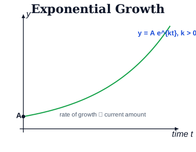
Drawn by us to help you understand the concept clearly, and verified to make sure it's accurate. For exams, practice from your NCERT textbook's own diagram.

Exponential growth: y = A e^(kt), k > 0 — the rate of increase is proportional to the …

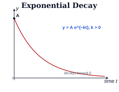
Figure 3.12bExponential decay curve y = A e^(-kt): the quantity falls and approaches zero as time increases

Fig. 3.12b — Exponential decay curve y = A e^(-kt): the quantity falls and approaches zero as time increases

Drawn by us to help you understand the concept clearly, and verified to make sure it's accurate. For exams, practice from your NCERT textbook's own diagram.

Exponential decay: y = A e^(−kt), k > 0 — the quantity decreases toward z …

Start your 14-day free trial to unlock the full solution →

← Previous · 5.12.1The Process of Mathematical Modeling Next · 5.12.3 →Population Growth