Mathematics · Ch 9 — Applications of Integration
Fundamental Theorems of Integral Calculus and their Applications
Fundamental Theorems of Integral Calculus and their Applications
Evaluating as a limit of Riemann sums (§9.2) is correct but tedious, even for a very simple . Newton and Leibniz, working independently at around the same time, devised a vastly easier method based on two celebrated theorems connecting a function to its anti-derivative. Together these are called the Fundamental Theorems of Integral Calculus, and they provide the bridge between differential calculus and integral calculus.
Theorem 9.1 (First Fundamental Theorem of Integral Calculus). If is continuous on and for , then — i.e. is an anti-derivative of .
Theorem 9.2 (Second Fundamental Theorem of Integral Calculus). If is continuous on and is any anti-derivative of , then .
Since is the value of the definite (Riemann) integral, adding any arbitrary constant to the anti-derivative cancels out of the difference — so, unlike an indefinite integral, no is needed when evaluating a definite integral. As shorthand, we write . The value of a definite integral is a unique real number.
Properties of definite integrals (all following from Theorem 9.2, stated here without proof except where a quick derivation illuminates the trick):
Property 1. — the definite integral does not depend on the name of the integration variable.
Property 2. — reversing the limits flips the sign.
Property 3. , — additivity over subintervals.
Property 4. , constants — linearity.
Property 5. If , then , where — this is what justifies evaluating a definite integral by substitution (Examples 9.8-9.19 all use this).
Property 6. .
Proof. Substitute , so ; when and when . Then (renaming , Property 1).
Setting in Property 6 gives the very frequently used special case .
Property 7. .
Proof. By Property 3, . In substitute : when ; when ; . So . Adding gives the result.
Property 8 (even functions). If , then .
Property 9 (odd functions). If , then .
Both Properties 8-9 proof idea: by Property 3, ; substitute in to get , which equals (even case, giving Property 8) or (odd case, cancelling the other piece to give Property 9).
Property 10. If , then — immediate from Property 7.
Property 11. If , then — also immediate from Property 7.
Property 12. If , then . …
![Fig. 9.6 — Fig. 9.6 — Graph of the step function $[x^{2}]$ on $[0,1.5]$: value $0$ on $[0,1)$, $1$ on $[1,\sqrt{2})$ and $2$ on $[\sqrt{2},1.5]$](/figures/applications-of-integration/greatest-integer-x-squared-step-fig-9-6.svg)
Drawn by us to help you understand the concept clearly, and verified to make sure it's accurate. For exams, practice from your textbook's own diagram.
What this figure shows. Fig. 9.6 — Graph of the step function on : value on , on and on $[\sq …
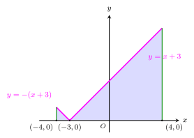
Drawn by us to help you understand the concept clearly, and verified to make sure it's accurate. For exams, practice from your textbook's own diagram.
What this figure shows. Fig. 9.7 — Graph of on : the branch for and for , vertex a …