Mathematics · Ch 8 — Differentials and Partial Derivatives
Limit and Continuity of Functions of Two Variables
Limit and Continuity of Functions of Two Variables
Definition 8.6 (Limit of a Function of Two Variables). Let and . has a limit at if: for every neighbourhood , , of , there exists a -neighbourhood of such that
We write if such a limit exists. All the standard limit theorems (limits of sums, differences, products, quotients — where the denominator's limit is nonzero — and composition with a continuous function) that hold for one-variable limits hold, unchanged in form, for functions of several variables.
Definition 8.7 (Continuity). is continuous at if: (1) is defined at ; (2) exists; and (3) that limit equals — the same three-part test as one variable, carried over verbatim.
The genuinely new subtlety compared to one variable: the values must approach the same as approaches along every possible path to — not only along straight lines, but along any curve whatsoever. This is what makes two-variable limits strictly harder to establish than one-variable limits (though, when a limit fails to exist, exhibiting just two disagreeing paths is enough to disprove it).
Worked example — a limit that fails to exist. Consider for , . Along any straight line through the origin,
a value that genuinely depends on the slope of the approach line — different lines through the origin give different limiting values (e.g. gives , gives ). Since the limit is not the same along every path, does not exist, and is consequently not continuous at .
Worked example — establishing continuity via a bound. Let for , ; this is continuous everywhere, including at the origin. Away from the origin it is a quotient of continuous functions with nonvanishing denominator, hence continuous there directly. At :
using . Since forces , the squeeze gives , so is continuous at too — hence continuous on all of .
Working method summary for a two-variable limit/continuity problem:
- Direct substitution whenever the expression is built from continuous pieces (polynomials, , , , , ...) combined algebraically or by composition, with any denominator nonzero at the target point. …
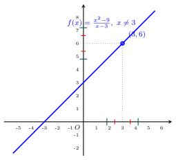
Drawn by us to help you understand the concept clearly, and verified to make sure it's accurate. For exams, practice from your textbook's own diagram.
What this figure shows. Fig. 8.7 — interplay of and for (the line with a hole at ); the limit as …
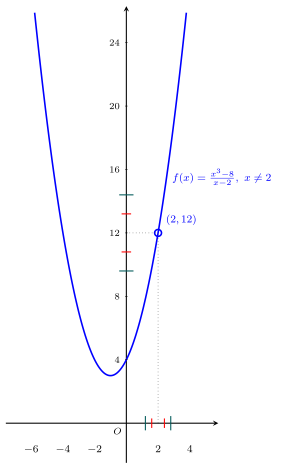
Drawn by us to help you understand the concept clearly, and verified to make sure it's accurate. For exams, practice from your textbook's own diagram.
What this figure shows. Fig. 8.8 — interplay of and for (the parabola with a hole at ); the limit as …
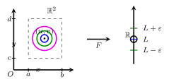
Drawn by us to help you understand the concept clearly, and verified to make sure it's accurate. For exams, practice from your textbook's own diagram.
What this figure shows. Fig 8.9 Limit of a function: a neighbourhood of (u,v) in the domain R^2 maps under F into the interval (L-e, L+e) on the real line, illustrati …
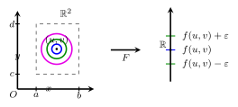
Drawn by us to help you understand the concept clearly, and verified to make sure it's accurate. For exams, practice from your textbook's own diagram.
What this figure shows. Fig 8.10 Continuity of a function: a neighbourhood of (u,v) maps under F into (f(u,v)-e, f(u,v)+e), with the limit value equa …