Skip to content

Mathematics · Ch 8 — Differentials and Partial Derivatives

Recall of Limit and Continuity of Functions of One Variable

8.3.1

Recall of Limit and Continuity of Functions of One Variable

Before extending limits and continuity to two variables, it helps to restate the one-variable definitions (from Class XI) in the language of neighbourhoods, since that is the form that generalizes cleanly.

Recall — Definition (Limit, one variable). f:(a,b)→Rf:(a,b)\to\mathbb R has limit LL at x0∈(a,b)x_0\in(a,b), written lim⁡x→x0f(x)=L\displaystyle\lim_{x\to x_0}f(x)=L, if: for every neighbourhood (L−ε,L+ε)(L-\varepsilon,L+\varepsilon), ε>0\varepsilon>0, of LL, there exists a neighbourhood (x0−δ,x0+δ)⊂(a,b)(x_0-\delta,x_0+\delta)\subset(a,b), δ>0\delta>0, of x0x_0, such that f(x)∈(L−ε,L+ε)f(x)\in(L-\varepsilon,L+\varepsilon) whenever x∈(x0−δ,x0+δ)∖{x0}x\in(x_0-\delta,x_0+\delta)\setminus\{x_0\}. Equivalently, in modulus notation: for every ε>0\varepsilon>0 there is δ>0\delta>0 such that ∣f(x)−L∣<ε|f(x)-L|<\varepsilon whenever 0<∣x−x0∣<δ0<|x-x_0|<\delta.

This is also characterised by matching one-sided limits: ff has a limit LL at x0x_0 (where ff is defined near, but not necessarily at, x0x_0) iff the right-hand limit L1=lim⁡x→x0+f(x)L_1=\lim_{x\to x_0^+}f(x) exists, the left-hand limit L2=lim⁡x→x0−f(x)L_2=\lim_{x\to x_0^-}f(x) exists, and L1=L2L_1=L_2 (then L=L1=L2L=L_1=L_2). Continuity at x0x_0 (where f(x0)f(x_0) is defined) additionally requires L=f(x0)L=f(x_0).

Neighbourhoods in the plane. The one-variable neighbourhood of x0∈Rx_0\in\mathbb R is the interval (x0−r,x0+r)(x_0-r,x_0+r), r>0r>0. To do the same for a point (u,v)∈R2(u,v)\in\mathbb R^2, define the rr-neighbourhood of (u,v)(u,v) as the open disc

Br((u,v))={(x,y)∈R2 ∣ (x−u)2+(y−v)2<r2},B_r((u,v)) = \big\{(x,y)\in\mathbb R^2 \ \big|\ (x-u)^2+(y-v)^2 < r^2\big\}, …

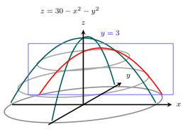
Figure 8.5Fig. 8.5 — the surface $z=30-x^{2}-y^{2}$ intersected by the plane $y=3$, whose cross-section is the parabola $g(x,3)=21-x^{2}$ (oblique 3D schematic)
Fig. 8.5 — Fig. 8.5 — the surface $z=30-x^{2}-y^{2}$ intersected by the plane $y=3$, whose cross-section is the parabola $g(x,3)=21-x^{2}$ (oblique 3D schematic)

Drawn by us to help you understand the concept clearly, and verified to make sure it's accurate. For exams, practice from your textbook's own diagram.

What this figure shows. Fig. 8.5 — the surface z=30−x2−y2z=30-x^{2}-y^{2} intersected by the plane y=3y=3, whose cross-section is the parabola g(x,3)=21−x2g(x,3)=21-x^{2} (oblique …

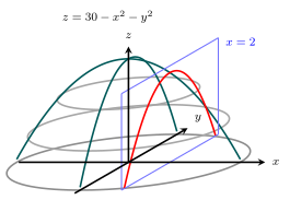
Figure 8.6Fig. 8.6 — the surface $z=30-x^{2}-y^{2}$ intersected by the plane $x=2$, whose cross-section is the parabola $g(2,y)=26-y^{2}$ (oblique 3D schematic)
Fig. 8.6 — Fig. 8.6 — the surface $z=30-x^{2}-y^{2}$ intersected by the plane $x=2$, whose cross-section is the parabola $g(2,y)=26-y^{2}$ (oblique 3D schematic)

Drawn by us to help you understand the concept clearly, and verified to make sure it's accurate. For exams, practice from your textbook's own diagram.

What this figure shows. Fig. 8.6 — the surface z=30−x2−y2z=30-x^{2}-y^{2} intersected by the plane x=2x=2, whose cross-section is the parabola g(2,y)=26−y2g(2,y)=26-y^{2} (oblique …