Skip to content

Mathematics · Ch 11 — Probability Distributions

Cumulative Distribution Function from Probability Mass function

11.3.4

Cumulative Distribution Function from Probability Mass function

Both the pmf and the cdf of a discrete random variable carry the same information — the full probability distribution is determined by either one. If XX takes the finitely many values x1<x2<⋯<xnx_1<x_2<\cdots<x_n, the cdf is built directly from the pmf as the running (cumulative) sum:

F(x)={0x<x1f(x1)x1≤x<x2f(x1)+f(x2)x2≤x<x3 ⋮f(x1)+⋯+f(xn)=1x≥xnF(x)=\begin{cases}0 & x<x_1\\ f(x_1) & x_1\le x<x_2\\ f(x_1)+f(x_2) & x_2\le x<x_3\\ \ \vdots & \\ f(x_1)+\cdots+f(x_n)=1 & x\ge x_n\end{cases}

For a discrete random variable XX, the cdf always satisfies six standing properties: (i) 0≤F(x)≤10\le F(x)\le1 for every xx; (ii) FF is real-valued and non-decreasing (x<y⇒F(x)≤F(y)x<y\Rightarrow F(x)\le F(y)); (iii) FF is right-continuous (lim⁡x→a+F(x)=F(a)\lim_{x\to a^+}F(x)=F(a)); (iv) lim⁡x→−∞F(x)=0\lim_{x\to-\infty}F(x)=0; (v) lim⁡x→∞F(x)=1\lim_{x\to\infty}F(x)=1; (vi) for x1<x2x_1<x_2, P(x1<X≤x2)=F(x2)−F(x1)P(x_1<X\le x_2)=F(x_2)-F(x_1); and consequently P(X>x1)=1−F(x1)P(X>x_1)=1-F(x_1). …

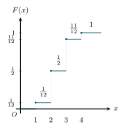
Figure 11.6Cumulative distribution function $F(x)$ (step function): $0$ for $x<1$, $\frac{1}{12}$ for $1\le x<2$, $\frac{1}{2}$ for $2\le x<3$, $\frac{11}{12}$ for $3\le x<4$, $1$ for $x\ge 4$ (Fig. 11.6)
Fig. 11.6 — Cumulative distribution function $F(x)$ (step function): $0$ for $x<1$, $\frac{1}{12}$ for $1\le x<2$, $\frac{1}{2}$ for $2\le x<3$, $\frac{11}{12}$ for $3\le x<4$, $1$ for $x\ge 4$ (Fig. 11.6)

Drawn by us to help you understand the concept clearly, and verified to make sure it's accurate. For exams, practice from your textbook's own diagram.

What this figure shows. Cumulative distribution function F(x)F(x) (step function): 00 for x<1x<1, 112\frac{1}{12} for 1≤x<21\le x<2, 12\frac{1}{2} for 2≤x<32\le x<3, 1112\frac{11}{12} for 3≤x<43\le x<4, 11 for $ …

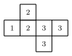
Figure 11.7Net of the special die marked $1$ on one face, $2$ on two faces and $3$ on three faces (used in the two-throw total-score example)
Fig. 11.7 — Net of the special die marked $1$ on one face, $2$ on two faces and $3$ on three faces (used in the two-throw total-score example)

Drawn by us to help you understand the concept clearly, and verified to make sure it's accurate. For exams, practice from your textbook's own diagram.

What this figure shows. Net of the special die marked 11 on one face, 22 on two faces and 33 on three faces (used in the two-throw total-scor …
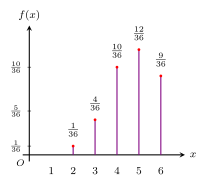
Figure 11.8Probability mass function of $f(x)$ for the total score in two throws of a die marked 1, 2, 2, 3, 3, 3: $f(2)=\frac{1}{36}$, $f(3)=\frac{4}{36}$, $f(4)=\frac{10}{36}$, $f(5)=\frac{12}{36}$, $f(6)=\frac{9}{36}$ (Fig. 11.8)
Fig. 11.8 — Probability mass function of $f(x)$ for the total score in two throws of a die marked 1, 2, 2, 3, 3, 3: $f(2)=\frac{1}{36}$, $f(3)=\frac{4}{36}$, $f(4)=\frac{10}{36}$, $f(5)=\frac{12}{36}$, $f(6)=\frac{9}{36}$ (Fig. 11.8)

Drawn by us to help you understand the concept clearly, and verified to make sure it's accurate. For exams, practice from your textbook's own diagram.

What this figure shows. Probability mass function of f(x)f(x) for the total score in two throws of a die marked 1, 2, 2, 3, 3, 3: f(2)=136f(2)=\frac{1}{36}, f(3)=436f(3)=\frac{4}{36}, f(4)=1036f(4)=\frac{10}{36}, f(5)=1236f(5)=\frac{12}{36}, $f(6)=\f …