Dielectrics and Polarisation

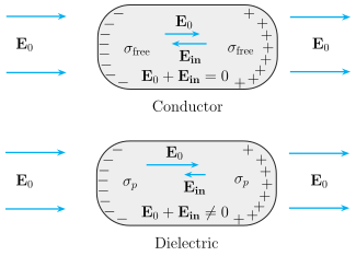
The figure is a side-by-side comparison of two identical slabs placed in the same uniform external electric field $\vec{E}_0$ (represented by long horizontal arrows entering from the left). The top slab is labelled Conductor, the bottom slab is labelled Dielectric.

What the figure shows

• External field: Both slabs experience the same uniform field $\vec{E}_0$ pointing to the right.
• Induced surface charges: On the left face of each slab, a layer of negative charge appears; on the right face, a layer of positive charge appears. For the conductor, these are labelled $\sigma_{\text{free}}$ (free charges). For the dielectric, they are labelled $\sigma_{\text{p}}$ (bound polarisation charges).
• Internal fields: Inside the conductor, there is an arrow for $\vec{E}_0$ (rightward) and a counter-arrow $\vec{E}_{\text{in}}$ (leftward) of equal length, with the annotation $E_0 + E_{\text{in}} = 0$ — the fields cancel exactly. Inside the dielectric, the opposing arrow $\vec{E}_{\text{in}}$ is shorter than $\vec{E}_0$, and the annotation reads $E_0 + E_{\text{in}} \neq 0$ — the cancellation is only partial.

The physical idea

The figure teaches the fundamental difference between conductors and dielectrics in an external field:

• In a conductor, free electrons move until the induced field exactly cancels the external field inside the material. The net field inside is zero.
• In a dielectric, charges are bound and cannot move freely. The external field only polarises the material — it stretches or rotates molecular dipoles, producing bound surface charges. These bound charges create an opposing field that reduces the external field but does not eliminate it. The net field inside the dielectric is non-zero but weaker than $\vec{E}_0$.

Key formula developed from this figure

The textbook uses this picture to define polarisation $\vec{P}$ (dipole moment per unit volume) and introduces the relation for linear isotropic dielectrics:

where:

• $\vec{P}$ = polarisation (dipole moment per unit volume, in $\text{C/m}^2$)
• $\varepsilon_0$ = permittivity of free space ($8.85 \times 10^{-12} \, \text{C}^2/\text{N·m}^2$)
• $\chi_e$ = electric susceptibility — a dimensionless constant characteristic of the dielectric material
• $\vec{E}$ = the net electric field inside the dielectric (not the external field $\vec{E}_0$) …

What the figure shows

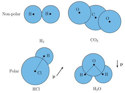
Fig. 2.21 presents ball-and-stick sketches of four molecules arranged in two rows. The top row shows non-polar molecules:

• H₂: two identical spheres labelled H–H, representing a symmetric diatomic molecule.
• CO₂: three collinear spheres O–C–O, representing a linear symmetric molecule.

The bottom row shows polar molecules:

• HCl: a large Cl sphere with a smaller H sphere attached at the upper-right, and a bold arrow labelled p pointing from Cl toward H (the dipole moment).
• H₂O: a large central O sphere with two H spheres attached at the lower-left and lower-right (bent shape), with a bold downward arrow labelled p marking the net dipole moment.

Physical idea taught by the figure

The figure illustrates the fundamental distinction between non-polar and polar molecules at the molecular level — a concept essential for understanding dielectrics.

• Non-polar molecules (top row) have their centres of positive and negative charges coinciding. Even though they contain charged particles, the symmetric arrangement (e.g., identical atoms in H₂, linear symmetry in CO₂) results in zero permanent dipole moment. In an external electric field, these molecules develop an induced dipole moment because the external field displaces positive and negative charges in opposite directions until internal restoring forces balance the external force.

• Polar molecules (bottom row) have a permanent dipole moment even in the absence of an external field. In HCl, the electronegativity difference between Cl and H shifts electron density toward Cl, creating a separation of charge. In H₂O, the bent geometry (bond angle ~104.5°) means the two O–H bond dipoles do not cancel; they add vectorially to give a net dipole moment (shown by the bold arrow p).

The figure directly supports the textbook’s explanation that when a dielectric is placed in an external electric field:

• For non-polar molecules, the field induces dipole moments.
• For polar molecules, the field aligns the existing permanent dipoles (overcoming thermal agitation).

In both cases, the dielectric develops a net dipole moment per unit volume, called polarisation $\mathbf{P}$.

Key formula developed with this figure

The textbook introduces the polarisation vector $\mathbf{P}$ and, for linear isotropic dielectrics, the relation:

where:

• $\mathbf{P}$ = dipole moment per unit volume (polarisation) of the dielectric.
• $\varepsilon_0$ = permittivity of free space ($8.85 \times 10^{-12} \, \text{C}^2/\text{N·m}^2$). …

What the Figure Shows

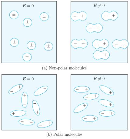
The figure is divided into two rows, each with two boxes. The top row is labelled (a) Non-polar molecules and the bottom row (b) Polar molecules. In each row, the left box is marked $E = 0$ (no external electric field) and the right box is marked $E \neq 0$ (external field present, directed to the right).

• Top row (a) – Non-polar molecules:

  In the left box ($E = 0$), you see several small circles, each with a coincident '$\pm$' symbol — meaning the positive and negative charge centres overlap exactly, so the molecule has zero permanent dipole moment.

  In the right box ($E \neq 0$), each molecule is stretched into a dumbbell shape: a '−' lobe on the left and a '+' lobe on the right. All these induced dipoles are aligned in the direction of the external field (rightward). This shows that the external field induces a dipole moment in each non-polar molecule by displacing charges.

• Bottom row (b) – Polar molecules:

  In the left box ($E = 0$), you see ovals with '−' and '+' ends pointing in random directions — each molecule has a permanent dipole moment, but thermal agitation makes their orientations random, so the net dipole moment of the whole sample is zero.

  In the right box ($E \neq 0$), the dipoles are roughly aligned: '−' on the left, '+' on the right, all pointing along the field. This shows that the external field reorients the permanent dipoles, producing a net dipole moment in the direction of the field.

Physical Idea Taught

The figure illustrates the two mechanisms by which a dielectric (insulator) develops a net dipole moment when placed in an external electric field:

1. For non-polar molecules: The field stretches the molecule, separating positive and negative charge centres, creating an induced dipole moment proportional to the field strength.
2. For polar molecules: The field exerts a torque on each permanent dipole, aligning them partially against thermal randomness, giving a net dipole moment in the field direction.

In both cases, the result is that the dielectric becomes polarised — it acquires a net dipole moment per unit volume, called the polarisation $\mathbf{P}$.

Key Formula Developed from This Figure

For linear isotropic dielectrics, the polarisation is directly proportional to the external electric field $\mathbf{E}$ inside the dielectric:

where:

• $\mathbf{P}$ = polarisation (dipole moment per unit volume, in $\text{C/m}^2$)
• $\varepsilon_0$ = permittivity of free space ($8.85 \times 10^{-12} \, \text{C}^2/\text{N·m}^2$)
• $\chi_e$ = electric susceptibility of the dielectric (a dimensionless constant that characterises how easily the material polarises) …

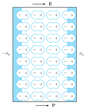
The figure shows a tall rectangular slab representing a uniformly polarised dielectric. Inside the slab, a regular grid of aligned horizontal dipoles is drawn — about 8 rows and 4 columns of small dumbbells. Each dumbbell has a '−' (negative) lobe on the left and a '+' (positive) lobe on the right, and all are parallel, pointing to the right.

Above the slab, a horizontal arrow labelled E points to the right — this is the external electric field applied to the dielectric. Below the slab, another horizontal arrow labelled P also points to the right — this is the polarisation (dipole moment per unit volume) induced in the dielectric.

At the left edge of the slab, a shaded strip is labelled $-\sigma_p$ — this is the induced negative surface charge density (bound charge). At the right edge, a shaded strip labelled $\sigma_p$ indicates the induced positive surface charge density. In the interior of the slab, the positive lobe of one dipole sits next to the negative lobe of the adjacent dipole, so the charges pair off and cancel — hence no net volume charge density inside.

---

Physical idea

The figure illustrates that when a uniform external field $\mathbf{E}_0$ is applied to a dielectric, the material becomes polarised: each molecular dipole aligns with the field. The net effect is that only the surfaces perpendicular to the field carry net charge — these are bound surface charges (not free charges). Inside the dielectric, the positive and negative charges of neighbouring dipoles cancel, so there is no net charge in the bulk. The induced surface charges produce an internal field opposite to $\mathbf{E}_0$, reducing the total field inside the dielectric.

---

Key formula developed from this figure

The polarisation $\mathbf{P}$ is defined as the dipole moment per unit volume. For a linear isotropic dielectric, it is proportional to the total electric field $\mathbf{E}$ inside the material:

where:

• $\mathbf{P}$ = polarisation (dipole moment per unit volume, in $\text{C/m}^2$)
• $\varepsilon_0$ = permittivity of free space ($8.85 \times 10^{-12} \, \text{C}^2/\text{N·m}^2$)
• $\chi_e$ = electric susceptibility of the dielectric (dimensionless constant)
• $\mathbf{E}$ = net electric field inside the dielectric (in $\text{N/C}$ or $\text{V/m}$) …