Physics · Ch 10 — Wave Optics

Polarisation

10.7

Polarisation

What is Polarisation?

Polarisation is a property unique to transverse waves — waves where the oscillation is perpendicular to the direction of propagation. Light waves are transverse: the electric field oscillates at right angles to the direction the wave travels. Polarisation describes the direction of that oscillation.

Understanding Polarisation with a String

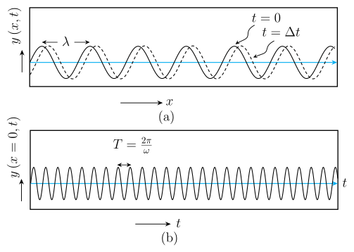
Imagine a long string held horizontally, with one end fixed. If you move the free end up and down periodically, a wave travels along the string in the $+x$ direction. The displacement of each point on the string is along the $y$ -axis. This is a transverse wave.

The displacement at any position $x$ and time $t$ is given by:

y(x,t) = a \sin(kx - \omega t)

where:

$a$ = amplitude of the wave
$\omega = 2\pi \nu$ = angular frequency ( $\nu$ is frequency)
$k = \frac{2\pi}{\lambda}$ = wave number ( $\lambda$ is wavelength)

Since the displacement is always along the $y$ -direction, this wave is called a $y$ -polarised wave. Because each point moves in a straight line (up and down), it is also called a linearly polarised wave. The entire string stays in the $x$ - $y$ plane, so it is a plane polarised wave.

Similarly, if you vibrate the string in the $x$ - $z$ plane, you get a $z$ -polarised wave:

z(x,t) = a \sin(kx - \omega t)

If the plane of vibration changes randomly in very short time intervals, the wave is unpolarised — the displacement direction changes randomly, but always remains perpendicular to the direction of propagation.

Polarisation of Light

Light waves are transverse — the electric field vector $\mathbf{E}$ oscillates perpendicular to the direction of propagation. Ordinary light (e.g., from the sun or a lamp) is unpolarised: the electric vector takes all possible directions in the transverse plane, rapidly and randomly.

How a Polaroid Works

A polaroid is a thin plastic sheet containing long-chain molecules aligned in a specific direction. When unpolarised light falls on it:

The component of the electric field parallel to the aligned molecules is absorbed.
The component perpendicular to the aligned molecules is transmitted.

The direction along which the electric vector oscillates after passing through the polaroid is called the pass-axis.

Effect of a Single Polaroid

When unpolarised light passes through a single polaroid, the transmitted intensity is half the incident intensity. Rotating the polaroid does not change this — the transmitted intensity remains constant.

Malus' Law: Light Through Two Polaroids

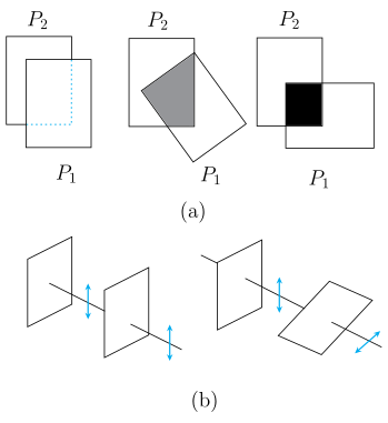
Place a second polaroid (P2) after the first (P1). The light emerging from P1 is linearly polarised along its pass-axis. If the pass-axis of P2 makes an angle $\theta$ with that of P1, only the component of the electric field parallel to P2's axis passes through.

The transmitted intensity $I$ is given by Malus' law:

I = I_0 \cos^2 \theta

where:

$I_0$ = intensity of polarised light after passing through the first polaroid
$\theta$ = angle between the pass-axes of the two polaroids

When $\theta = 0^\circ$ , $I = I_0$ (maximum transmission).

When $\theta = 90^\circ$ , $I = 0$ (no transmission — crossed polaroids).

Controlling Intensity with Two Polaroids

By rotating one polaroid relative to the other, the transmitted intensity can be varied continuously from 50% (when only one polaroid is used) down to 0% of the incident intensity.

Example: Rotating a Polaroid Between Two Crossed Polaroids

Let P1 and P3 be crossed (pass-axes at $90^\circ$ ). Place P2 between them, with its pass-axis at an angle $\theta$ to P1.

Intensity after P1: $I_0$ …

Figure 10.17(a) The curves represent the displacement of a string at t = 0 and at t = Δt, respectively when a sinusoidal wave is propagating in the +x-direction. (b) The curve represents the time variation of the displacement at x = 0 when a sinusoidal wave is propagating in the +x-direction. At x = Δx, the time variation of the displacement will be slightly displaced to the right.

Fig. 10.17 — (a) The curves represent the displacement of a string at t = 0 and at t = Δt, respectively when a sinusoidal wave is propagating in the +x-direction. (b) The curve represents the time variation of the displacement at x = 0 when a sinusoidal wave is propagating in the +x-direction. At x = Δx, the time variation of the displacement will be slightly displaced to the right.

Drawn by us to help you understand the concept clearly, and verified to make sure it's accurate. For exams, practice from your NCERT textbook's own diagram.

Figure 10.17 is a two‑panel diagram that introduces the idea of a linearly polarised transverse wave on a string, which is then used as a model for light waves.

Panel (a): Displacement vs. Position (Snapshot at Two Times)

Axes: The horizontal axis is position $x$ along the string; the vertical axis is displacement $y$ (perpendicular to $x$ ).
Curves: Two identical sine curves are drawn. One is labelled $t = 0$ (the wave at the initial instant). The other is labelled $t = \Delta t$ (a short time later). The second curve is shifted to the right along the $x$ ‑axis by a small amount.
Physical idea: The rightward shift shows that the wave pattern moves in the $+x$ direction as time increases. Each point on the string oscillates up and down (transverse motion), but the shape of the wave travels forward.
Key label: An arrow marked $+x$ direction indicates the direction of propagation.

Panel (b): Displacement vs. Time (Fixed Position)

Axes: The horizontal axis is time $t$ ; the vertical axis is displacement $y$ (again perpendicular to $x$ ).
Curve: A sine curve showing how the displacement at a fixed point (say $x = 0$ ) varies with time.
Physical idea: If you sit at one location on the string, you see the string move up and down sinusoidally as the wave passes. The text notes that at a different fixed point $x = \Delta x$ , the same time‑variation curve would be slightly displaced to the right — meaning the oscillation at that point is delayed (a phase lag) because the wave takes time to travel from $x = 0$ to $x = \Delta x$ .

The Key Formula Developed from This Figure

The wave shown in both panels is described by the sinusoidal travelling wave equation:

y(x,t) = a \sin(kx - \omega t)

where:

$y(x,t)$ is the displacement of the string at position $x$ and time $t$ (perpendicular to $x$ ).
$a$ is the amplitude — the maximum displacement from equilibrium.
$\omega = 2\pi \nu$ is the angular frequency ( $\nu$ is the ordinary frequency).
$k = \frac{2\pi}{\lambda}$ is the wave number, with $\lambda$ the wavelength. …

Figure 10.18(a) Passage of light through two polaroids P2 and P1. The transmitted fraction falls from 1 to 0 as the angle between them varies from 0° to 90°. Notice that the light seen through a single polaroid P1 does not vary with angle. (b) Behaviour of the electric vector when light passes through two polaroids. The transmitted polarisation is the component parallel to the polaroid axis. The double arrows show the oscillations of the electric vector.

$Fig. 10.18 — (a) Passage of light through two polaroids P2 and P1. The transmitted fraction falls from 1 to 0 as the angle between them varies from 0° to 90°. Notice that the light seen through a single polaroid P1 does not vary with angle. (b) Behaviour of the electric vector when light passes through two polaroids. The transmitted polarisation is the component parallel to the polaroid axis. The double arrows show the oscillations of the electric vector.$

Drawn by us to help you understand the concept clearly, and verified to make sure it's accurate. For exams, practice from your NCERT textbook's own diagram.

What Figure 10.18 Shows

The figure has two panels, (a) and (b), that together illustrate how polarisation controls light intensity.

Panel (a) is a schematic diagram showing the experimental setup. Unpolarised light (from a lamp) first passes through a polaroid labelled P2. After P2, the light becomes plane polarised — its electric field oscillates only along the pass-axis of P2. This polarised beam then encounters a second polaroid P1, whose pass-axis can be rotated to make an angle $\theta$ with that of P2. The transmitted intensity after P1 is plotted as a function of $\theta$ : it is maximum (full intensity) when $\theta = 0^\circ$ , and falls to zero when $\theta = 90^\circ$ . The caption notes that if only a single polaroid (say P1) is used, rotating it does not change the transmitted intensity — it remains constant at half the incident intensity.

Panel (b) is a vector diagram that explains why the intensity varies. It shows the electric field vector E (represented by a double-headed arrow) oscillating along the pass-axis of P2. The pass-axis of P1 is drawn at an angle $\theta$ to this direction. The component of E that is parallel to P1’s axis is $E \cos\theta$ — this is the part that gets transmitted. The perpendicular component $E \sin\theta$ is absorbed. The transmitted intensity is proportional to the square of this component.

Physical Idea

The figure demonstrates Malus’ law for polarised light. When plane-polarised light passes through a second polaroid (called an analyser), only the component of the electric field parallel to the analyser’s pass-axis is transmitted. Rotating the analyser changes the fraction of the field that passes through, and since intensity is proportional to the square of the field amplitude, the transmitted intensity varies as $\cos^2\theta$ .

Key Formula

The textbook derives Malus’ law from this figure:

I = I_0 \cos^2\theta

where:

$I$ is the intensity of light transmitted through the second polaroid (P1),
$I_0$ is the intensity of the plane-polarised light incident on P1 (i.e., after P2),
$\theta$ is the angle between the pass-axes of the two polaroids. …

Start your 14-day free trial to unlock the full solution →

← Previous · 10.6.2Seeing the Single Slit Diffraction Pattern Next · 10.7 →Example 10.2 — Discuss the intensity of transmitted light when a polaroid sheet is ro…