Biology · Ch 13 — Plant Growth and Development
Growth Rates
Growth Rates
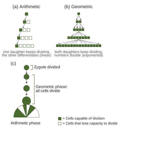
The increased growth per unit time is termed the growth rate. The rate of growth can be expressed mathematically, because an organism, or a part of an organism, can produce more cells in a variety of ways. The increase shown by the growth rate may be arithmetic or geometrical.
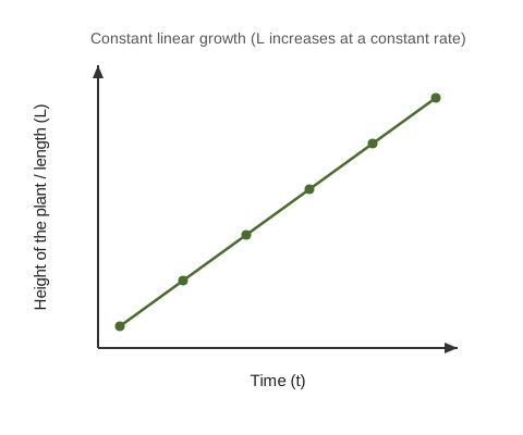
- Arithmetic growth — Following mitotic cell division, only one daughter cell continues to divide while the other differentiates and matures. The simplest example is a root elongating at a constant rate. On plotting the length of the organ against time, a linear curve is obtained. Mathematically it is expressed as Lt = L0 + rt, where Lt is the length at time t, L0 is the length at time zero, and r is the growth rate or elongation per unit time.
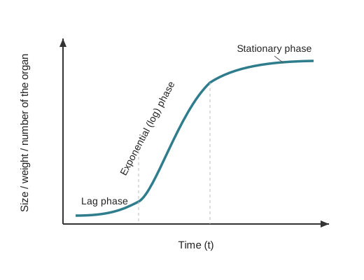
- Geometric growth — In most systems the initial growth is slow (the lag phase) and then increases rapidly at an exponential, or log, rate. Here both progeny cells following mitotic division retain the ability to divide and continue to do so. However, with a limited nutrient supply, growth eventually slows down, leading to a stationary phase. On plotting the parameter of growth against time, a typical sigmoid or S-curve is obtained. This curve, with its lag, exponential and stationary phases, is a characteristic of living organisms growing in a natural environment and is typical of all cells, tissues and organs of a plant.
Exponential growth can be expressed as W1 = W0 e raised to the power rt, where W1 is the final size, W0 is the initial size at the beginning of the period, r is the growth rate, t is the time of growth, and e is the base of natural logarithms. Here r is the relative growth rate and is also a measure of the ability of the plant to produce new plant material, referred to as the efficiency index; the final size W1 therefore depends on the initial size W0.
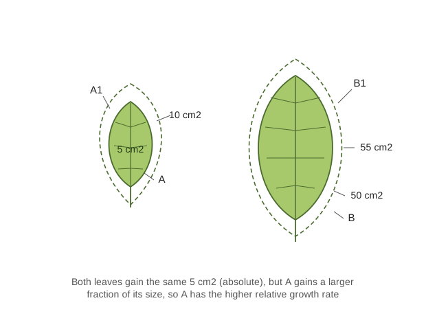
Quantitative comparisons between the growth of living systems can also be made in two ways. …
Drawn by us to help you understand the concept clearly, and verified to make sure it's accurate. For exams, practice from your textbook's own diagram.
This figure compares the two patterns in which cells can multiply during growth. In part (a), arithmetic growth, only one of the two daughter cells continues to divide after each division while the other stops and matures, so the number of dividing cells stays the same; a key distinguishes cells still capable of division from those that have lost the capacity. In part (b), geometric growth, both daughter cells keep dividing, so the number of dividing cells multiplies rapidly at each step. Part (c) applies these ideas to a developing embryo starting from the divided zygote: an early geometric phase, in which all cells divide, is followed by an arithmetic phase, in which cells at the periphery progressively lose the ability to di …
Drawn by us to help you understand the concept clearly, and verified to make sure it's accurate. For exams, practice from your textbook's own diagram.
This graph shows what arithmetic, or linear, growth looks like when plotted. The length of the plant (L) is placed on the vertical axis and time (t) on the horizontal axis. As time passes, the plotted points rise in a straight line, meaning that equal amounts of length are added in equal intervals of time — the growth rate stays constant. This is exactly the pattern produced by a root elongating at a constant rate, where only one daughter cell continues to divide after each division. The straight-line relationship corresponds to the expression Lt = L0 + rt, in which L0 is the length at the start, r is the constant elongation per unit time, and Lt is the …
Drawn by us to help you understand the concept clearly, and verified to make sure it's accurate. For exams, practice from your textbook's own diagram.
This graph shows the characteristic S-shaped, or sigmoid, curve obtained when the size or weight of an organ is plotted against time during geometric growth. The curve has three clear parts. It begins with a slow lag phase, where growth is only just getting under way. It then rises steeply through the exponential (log) phase, during which both progeny cells keep dividing and the organ grows very rapidly. Finally, as the nutrient supply becomes limiting, the curve levels off into a stationary phase, where growth slows and almost stops. This sigmoid pattern is typical of cells growing in culture and of many higher plants and plant organs growing in a natural environment, which is why it is regarded as a ch …
Drawn by us to help you understand the concept clearly, and verified to make sure it's accurate. For exams, practice from your textbook's own diagram.
This figure explains the difference between absolute and relative growth rates using two leaves of different sizes. A small leaf A and a larger leaf B each add the same absolute increase in area, 5 square centimetres, in the same period of time, becoming leaves A1 and B1 (the small leaf grows from 5 to 10, the large one from 50 to 55). Because both add the same total area per unit time, their absolute growth rates are equal. However, when the increase is expressed on a common basis, such as per unit of the leaf's own initial area, the picture changes: the smaller leaf A shows a much higher relative growth rate, because 5 square centimetres is a far larger fraction …