Shapes of Atomic Orbitals

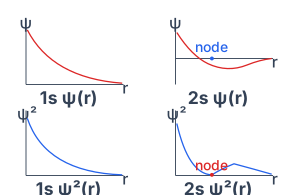
Fig. 2.12 is a set of four plots that show how the wave function $\psi(r)$ (top row) and the probability density $\psi^2(r)$ (bottom row) behave as you move away from the nucleus along a radial line $r$, for the 1s orbital (left) and the 2s orbital (right).

In the top row, the 1s curve starts at a high positive value right at the nucleus ($r=0$) and then decays smoothly toward zero as $r$ increases — no sign change, no bumps. The 2s curve also starts positive, but it does something the 1s curve does not: it crosses zero (the point marked node in the plot), goes negative, and then returns toward zero from below. That crossing point is a radial node — a spherical shell where the wave function is exactly zero.

The bottom row shows $\psi^2(r)$ for the same orbitals. The 1s curve begins at a very high value at $r=0$ and decays monotonically. The 2s curve starts high, drops to zero at the same radial node, rises to a small local maximum, and then decays to zero. The key point: $\psi^2(r)$ is never negative — it is always zero or positive, because it is a squared quantity.

The physical idea this figure teaches is that the wave function $\psi$ can have positive and negative regions, but the probability of finding the electron — given by $\psi^2$ — is always non-negative. The node is a spherical surface where the electron is never found. The 1s orbital has no such surface; the electron can be found anywhere (with decreasing probability as $r$ increases). The 2s orbital has one spherical shell of zero probability.

The central formula that the textbook develops with this figure is the relationship between the wave function and probability density:

Here $P(r) \, dV$ is the probability of finding the electron in a small volume element $dV$ at a distance $r$ from the nucleus. $|\psi(r)|^2$ is the probability density — the probability per unit volume. The figure shows that for the 1s orbital, this probability density is maximum at the nucleus and falls off smoothly. For the 2s orbital, it drops to zero at the node, then rises again before finally decaying.

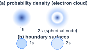
Fig. 2.13 is the first visual bridge between the abstract wavefunction $\psi$ and the concrete picture of an orbital that you can hold in your mind. It shows two different ways of representing the same quantum object: the 1s and 2s orbitals of hydrogen.

Panel (a) — Probability density plots. These are electron-cloud pictures: the depth of shading at any point is proportional to $|\psi|^2$, the probability density (the book's own version builds the same picture out of individual dots). For the 1s orbital the cloud is darkest at the nucleus and fades smoothly outward — a single spherical cloud with no gap; the probability is highest at the centre and decreases monotonically.

For the 2s orbital, the picture is strikingly different. Close to the nucleus there is a dense inner cloud. Then, at a certain distance, a spherical shell appears where the shading vanishes completely — the nodal region (labelled in the figure). Beyond that node, a second, outer shell of cloud appears, fainter than the inner region but clearly present. This is the first direct visual evidence that $|\psi|^2$ can go to zero at a finite distance from the nucleus, even though the electron is still bound to the atom.

Panel (b) — Boundary surface diagrams. These are simplified, practical representations. Instead of showing every dot, we choose a constant-$|\psi|^2$ surface that encloses about 90% of the total probability of finding the electron. For the 1s orbital, that surface is a single sphere. For the 2s orbital, the boundary surface is also a sphere, but it is larger than the 1s sphere. The key point: the boundary surface diagram of the 2s orbital does not show the internal node — it only shows the outer envelope. The node is invisible in this representation, which is why the textbook explicitly labels the "nodal region" in panel (a) but not in panel (b).

The physical idea this figure teaches is profound: orbitals are not fixed paths. The electron does not orbit the nucleus like a planet. Instead, the orbital is a region of space where the electron is likely to be found, and that region can have internal structure — including nodes where the probability is exactly zero. The 2s orbital has one radial node; the 1s orbital has none. In general, an ns orbital has $(n-1)$ radial nodes.

The central formula that connects the figure to the theory is the definition of probability density:

where $\psi(r)$ is the wavefunction (the atomic orbital) and $P(r)$ is the probability density at a distance $r$ from the nucleus. The dot-density in panel (a) is a visual representation of $P(r)$. The boundary surface in panel (b) is drawn at a value of $|\psi|^2$ such that the volume integral of $P(r)$ over the enclosed region equals 0.9 (or 90%).

For the 1s orbital, the wavefunction is:

where $a_0$ is the Bohr radius ($\approx 0.529 \text{ Å}$). This function is positive everywhere and decays exponentially — no nodes.

For the 2s orbital, the wavefunction has a radial node:

The factor $(2 - r/a_0)$ changes sign at $r = 2a_0$, making $\psi_{2s} = 0$ there. Since $|\psi|^2$ is the square, the probability density is zero at that radius — that is the nodal region you see in the dot-density plot. …

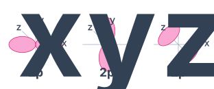
The figure shows three separate coordinate systems, each with a single dumbbell-shaped orbital drawn through the origin. Each dumbbell has two identical lobes, one on each side of the nucleus, and the nucleus sits at the centre where the axes cross. The three orbitals are labelled $2p_x$, $2p_y$, and $2p_z$, and each one is aligned along a different axis: $2p_x$ lies along the x-axis, $2p_y$ along the y-axis, and $2p_z$ along the z-axis. The axes themselves are labelled $x$, $y$, $z$ in the usual right-handed orientation.

The key physical idea is that a $2p$ orbital is not a spherical cloud like an $s$ orbital. Instead, it has a directional shape with two lobes and a nodal plane that passes through the nucleus. For $2p_x$, the nodal plane is the $yz$-plane; for $2p_y$, it is the $xz$-plane; for $2p_z$, it is the $xy$-plane. On that plane, the probability of finding the electron is exactly zero. The lobes themselves represent regions where the wave function $\psi$ has opposite signs — one lobe is positive, the other negative — but the probability density $|\psi|^2$ is the same in both lobes because squaring removes the sign.

The figure directly illustrates the quantum numbers that arise from solving the Schrödinger equation for the hydrogen atom. The principal quantum number $n = 2$ tells us this is the second energy level. The azimuthal quantum number $l = 1$ (for a $p$ orbital) gives the orbital its dumbbell shape. The magnetic quantum number $m_l$ takes three values: $m_l = -1, 0, +1$, which correspond to the three orientations $2p_x$, $2p_y$, and $2p_z$ respectively. So the three diagrams are not three different kinds of orbitals — they are the same orbital type ($2p$) pointing in three perpendicular directions.

The textbook uses this figure to make a deeper point about the quantum mechanical model. Unlike Bohr's model, which pictured the electron moving in fixed circular orbits, quantum mechanics gives us only a probability distribution. The boundary surface diagram is a visual summary of that distribution: it shows where the electron is most likely to be found, not a path it follows. The nodal plane is a direct consequence of the wave nature of the electron — it is a region where the wave function $\psi$ changes sign and therefore must be zero. …

The five diagrams in Fig. 2.15 are boundary surface diagrams of the 3d orbitals. They are not photographs of an electron; they are a visual representation of the region in space where there is a 90–95% probability of finding the electron that occupies that orbital. The axes (x, y, z) are drawn through the nucleus at the origin.

Each orbital has a characteristic shape determined by its angular part. The four orbitals $3d_{xy}$, $3d_{xz}$, $3d_{yz}$, and $3d_{x^2-y^2}$ each show four lobes arranged in a cloverleaf pattern. The key difference is the orientation of the lobes relative to the coordinate axes. For $3d_{xy}$, the four lobes lie between the x and y axes; for $3d_{xz}$, between x and z; for $3d_{yz}$, between y and z. The $3d_{x^2-y^2}$ orbital also has four lobes, but they lie along the x and y axes themselves. The $3d_{z^2}$ orbital is different: it has two lobes along the z-axis (one above, one below the nucleus) and a doughnut-shaped ring (a torus) lying in the xy-plane around the nucleus.

The physical idea is that an atomic orbital is not a fixed orbit like a planet's path. It is a probability cloud described by the wave function $\psi$. The square of the wave function, $|\psi|^2$, gives the probability density at any point. The boundary surface encloses the volume where the probability of finding the electron is, say, 90%. The shape of this surface is determined by the angular part of the wave function, which depends on the quantum numbers $l$ and $m_l$. For $l=2$ (d orbitals), the angular part has a specific mathematical form that produces these cloverleaf and dumbbell-with-ring shapes.

The central formula that connects the figure to the theory is the Schrödinger equation for the hydrogen atom. Its solution yields the wave function $\psi_{n,l,m_l}(r,\theta,\phi)$, which can be separated into a radial part $R_{n,l}(r)$ and an angular part $Y_{l,m_l}(\theta,\phi)$:

Here:

• $n$ is the principal quantum number (energy level).
• $l$ is the azimuthal quantum number (orbital shape; for d orbitals, $l=2$).
• $m_l$ is the magnetic quantum number (orbital orientation; takes values $-2, -1, 0, +1, +2$ for $l=2$).
• $r$, $\theta$, $\phi$ are the spherical coordinates of the electron relative to the nucleus.
• $R_{n,l}(r)$ describes how the probability density varies with distance from the nucleus.
• $Y_{l,m_l}(\theta,\phi)$ describes the angular shape — it is this part that gives the cloverleaf or dumbbell-with-ring pattern.

The boundary surface diagram is essentially a plot of the angular part $|Y_{l,m_l}(\theta,\phi)|^2$ at a fixed radial distance where the probability density is high. The five diagrams correspond to the five possible values of $m_l$ for $l=2$: $m_l = -2, -1, 0, +1, +2$. The textbook labels them as $3d_{xy}$, $3d_{xz}$, $3d_{yz}$, $3d_{x^2-y^2}$, and $3d_{z^2}$ — these are the real combinations of the complex spherical harmonics that are easier to visualize. …