Short Run Equilibrium of the Monopoly Firm

As with perfect competition, we treat the monopoly firm as a profit maximiser, and we assume it keeps no stocks — the whole output produced is put up for sale. We work out the equilibrium in three ways: a simple zero-cost case, the total-curves method, and the average-and-marginal-curves method.

The simple case of zero cost

Imagine a village, far from other villages, with exactly one well that supplies all the water. The well is owned by one person who can stop anyone else drawing water except by purchase, and buyers draw the water out themselves. The owner is therefore a monopolist who bears zero cost in producing the good.

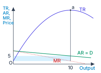
Profit equals revenue minus cost: $\text{Profit} = TR - TC$. Since here $TC = 0$, profit is greatest exactly where $TR$ is greatest — at 10 units, the output at which $MR = 0$ (Fig. 6.6). The price is whatever consumers as a whole are willing to pay for 10 units, read off the demand curve: Rs 5. Because the demand curve is the $AR$ curve, Rs 5 is the average revenue, and total revenue is $AR \times q = 5 \times 10 = \text{Rs } 50$, shown by the shaded rectangle.

Comparison with perfect competition. Now suppose there were an infinite number of such wells. If one owner charged Rs 5 a bucket, another could undercut him at Rs 4, a third at a still lower price, and so on — competition among owners would drive the price down to zero, at which 20 buckets would be sold. So a perfectly competitive equilibrium yields a larger quantity at a lower price than a monopoly. We now turn to the general case with positive costs.

Introducing positive costs — analysing with total curves

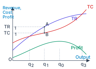
Using the S-shaped total cost curve $TC$ from the theory of costs, drawn together with the $TR$ curve (Fig. 6.7), profit is the vertical distance between $TR$ and $TC$. At output $q_1$, profit is $TR_1 - TC_1$, shown by the segment $AB$. This distance changes with output: when output is below $q_2$, $TC$ lies above $TR$ and the firm makes losses; the same is true above $q_3$. The firm can make positive profits only between $q_2$ and $q_3$, where $TR$ lies above $TC$. It chooses the output at which $TR - TC$ is maximum — output $q_0$, where the Profit curve (drawn as $TR - TC$) reaches its peak. The price charged is the price consumers will pay for $q_0$, read off the demand curve.

Using average and marginal curves

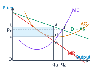
The same result comes out more sharply using the Average Cost ($AC$), Average Variable Cost ($AVC$) and Marginal Cost ($MC$) curves drawn with the demand ($AR$) and marginal revenue ($MR$) curves (Fig. 6.8). Below $q_0$, $MR$ exceeds $MC$: an extra unit adds more to revenue than to cost, so producing it increases profit — the firm expands as long as $MR > MC$. Above $q_0$, $MC$ exceeds $MR$: cutting a unit saves more cost than the revenue lost, so the firm contracts as long as $MC > MR$. The firm stops adjusting where $MR = MC$. Hence the equilibrium condition for a monopoly firm is $MR = MC$ (with $MC$ rising), which fixes the equilibrium output $q_0$; the equilibrium price is then read off the demand curve at $q_0$.

At $q_0$, average cost is the height $dq_0$ (point 'd' on the $AC$ curve), so total cost is the rectangle $Oq_0dc$; price is the height $aq_0$ (point 'a' on the demand curve), so total revenue is the rectangle $Oq_0ab$. Because $Oq_0ab$ is larger than $Oq_0dc$, $TR > TC$, and the profit is the rectangle $cdab$.

Comparison with perfect competition again

If the same firm behaved as a price taker (believing it could not change price by altering output), it would keep expanding as long as price exceeded $MC$, stopping only where price = $MC$, at point 'f' where the $MC$ curve cuts the demand curve. That gives a larger output $q_c$ and a lower price $p_c$ than the monopoly's $q_0$ and price. So, compared with monopoly, perfect competition sells a larger quantity at a lower price, and the perfectly competitive firm's profit is smaller.

In the long run

With free entry and exit, perfectly competitive firms earn zero profit in the long run — positive profits attract entry (raising output, lowering price) and losses cause exit (lowering output, raising price) until profit is wiped out. A monopoly is different: because other firms are barred from entering, a monopolist's positive profits do not disappear in the long run.

Some critical views …