Skip to content

Chemistry · Ch 6 — Chemical Kinetics

Zero order reactions

6.5.8

Zero order reactions

The rate of a zero order reaction is independent of the reactant concentration.

Integrated rate law for zero order reactions : For the zero order reaction

A⟶P\mathrm{A \longrightarrow P}

the differential rate law is given by

rate=−d[A]dt=k [A]0=k...(6.14)\text{rate} = -\frac{\mathrm{d[A]}}{\mathrm{d}t} = k\,\mathrm{[A]^0} = k \qquad \text{...(6.14)}

Rearrangement of Eq. (6.14) gives d[A]=−k dt\mathrm{d[A]} = -k\,\mathrm{d}t. Integration between the limits [A]=[A]0\mathrm{[A]} = \mathrm{[A]_0} at t=0t = 0 and [A]=[A]t\mathrm{[A]} = \mathrm{[A]_t} at t=tt = t gives

∫[A]0[A]td[A]=−k∫0tdt\int_{\mathrm{[A]_0}}^{\mathrm{[A]_t}} \mathrm{d[A]} = -k\int_0^t \mathrm{d}t

or [A]t−[A]0=−kt\text{or } \mathrm{[A]_t} - \mathrm{[A]_0} = -kt

Hence, kt=[A]0−[A]t...(6.15)\text{Hence, } kt = \mathrm{[A]_0} - \mathrm{[A]_t} \qquad \text{...(6.15)}

Units of rate constant of zero order reactions

k=[A]0−[A]tt=mol L−1t=mol dm−3 t−1k = \frac{\mathrm{[A]_0} - \mathrm{[A]_t}}{t} = \frac{\mathrm{mol\ L^{-1}}}{t} = \mathrm{mol\ dm^{-3}\ t^{-1}}

The units of the rate constant of a zero order reaction are the same as those of the rate itself.

Half life of zero order reactions : The rate constant of a zero order reaction is given by Eq. (6.15):

k=[A]0−[A]ttk = \frac{\mathrm{[A]_0} - \mathrm{[A]_t}}{t}

Using the conditions t=t1/2t = t_{1/2}, [A]t=[A]1/2=[A]0/2\mathrm{[A]_t} = \mathrm{[A]_{1/2}} = \mathrm{[A]_0}/2, Eq. (6.15) becomes

k=[A]0−[A]0/2t1/2=[A]02 t1/2k = \frac{\mathrm{[A]_0} - \mathrm{[A]_0}/2}{t_{1/2}} = \frac{\mathrm{[A]_0}}{2\,t_{1/2}}

Hence, t1/2=[A]02k...6.16\text{Hence, } t_{1/2} = \frac{\mathrm{[A]_0}}{2k} \qquad \text{...6.16}

The half life of a zero order reaction is proportional to the initial concentration of the reactant.

Graphical representation of zero order reactions : The rate law in Eq. (6.15) gives

[A]t=−kt+[A]0...6.17\mathrm{[A]_t} = -kt + \mathrm{[A]_0} \qquad \text{...6.17}

which is a straight line given by y=mx+cy = mx + c — the book's term-by-term arrows map [A]t\mathrm{[A]_t} to yy, −k-k to the slope mm, tt to xx and [A]0\mathrm{[A]_0} to the intercept cc. A plot of [A]t\mathrm{[A]_t} versus tt is a straight line, as shown in Fig. 6.6.
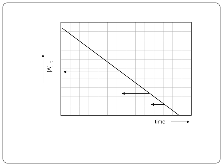
Figure 6.6Straight-line decrease of reactant concentration with time for a zero order reaction, falling from the initial concentration on the y-axis with slope minus k, with arrows showing the successive half lives shrinking as the reactant runs down.
Fig. 6.6 — Straight-line decrease of reactant concentration with time for a zero order reaction, falling from the initial concentration on the y-axis with slope minus k, with arrows showing the successive half lives shrinking as the reactant runs down.

Drawn by us to help you understand the concept clearly, and verified to make sure it's accurate. For exams, practice from your textbook's own diagram.

What this figure shows. For a zero order reaction Eq. 6.17, [A]t=−kt+[A]0\mathrm{[A]_t} = -kt + \mathrm{[A]_0}, plots as a straight line: it starts at [A]0\mathrm{[A]_0} on the y-axis and falls with slope −k-k until the reactant is exhausted. The left-pointing arrows mark successive halving spans — notice they get shorter toward the bottom: unlike a first order reaction, the half life here is proportional to the rema …

The slope of the straight line is −k-k and its intercept on the y-axis is [A]0\mathrm{[A]_0}. The t1/2t_{1/2} of a zero order reaction is directly proportional to the initial concentration.

Note

The printed tags of equations 6.16 and 6.17 (and 6.18 in section 6.7.1) appear in the book without the parentheses every other equation tag carries — "............ 6.16" rather than "(6.16)". The tags above follow the print.

Examples of zero order reactions :

Here follow some examples.

Decomposition of NH3\mathrm{NH_3} on platinum metal

2 NH3(g)⟶N2(g)+3 H2(g)\mathrm{2\,NH_3(g) \longrightarrow N_2(g) + 3\,H_2(g)} …